Causal Modeling in R: Whole Game

Malcolm Barrett

2021-09-01

1. Specify causal question (e.g. target trial)
2. Draw assumptions (causal diagram)
3. Model assumptions (e.g. propensity score)
4. Analyze propensities (diagnostics)
5. Estimate causal effects (e.g. IPW)
6. Sensitivity analysis (more later!)

We’ll focus on the broader ideas behind each step and what they look like all together; we don’t expect you to fully digest each idea. We’ll spend the rest of the workshop taking up each step in detail

Do people who quit smoking gain weight?

library(causaldata)
nhefs_complete_uc <- nhefs_complete |>
  filter(censored == 0)
nhefs_complete_uc

# A tibble: 1,566 × 67
    seqn  qsmk death yrdth modth dadth   sbp   dbp sex  
   <dbl> <dbl> <dbl> <dbl> <dbl> <dbl> <dbl> <dbl> <fct>
 1   233     0     0    NA    NA    NA   175    96 0    
 2   235     0     0    NA    NA    NA   123    80 0    
 3   244     0     0    NA    NA    NA   115    75 1    
 4   245     0     1    85     2    14   148    78 0    
 5   252     0     0    NA    NA    NA   118    77 0    
 6   257     0     0    NA    NA    NA   141    83 1    
 7   262     0     0    NA    NA    NA   132    69 1    
 8   266     0     0    NA    NA    NA   100    53 1    
 9   419     0     1    84    10    13   163    79 0    
10   420     0     1    86    10    17   184   106 0    
# ℹ 1,556 more rows
# ℹ 58 more variables: age <dbl>, race <fct>, income <dbl>,
#   marital <dbl>, school <dbl>, education <fct>, …

Did those who quit smoking gain weight?

Did those who quit smoking gain weight?

# ~2.5 KGs gained for quit vs. not quit
nhefs_complete_uc |>
  group_by(qsmk) |>
  summarize(
    mean_weight_change = mean(wt82_71), 
    sd = sd(wt82_71),
    .groups = "drop"
  )

# A tibble: 2 × 3
   qsmk mean_weight_change    sd
  <dbl>              <dbl> <dbl>
1     0               1.98  7.45
2     1               4.53  8.75

draw your assumptions

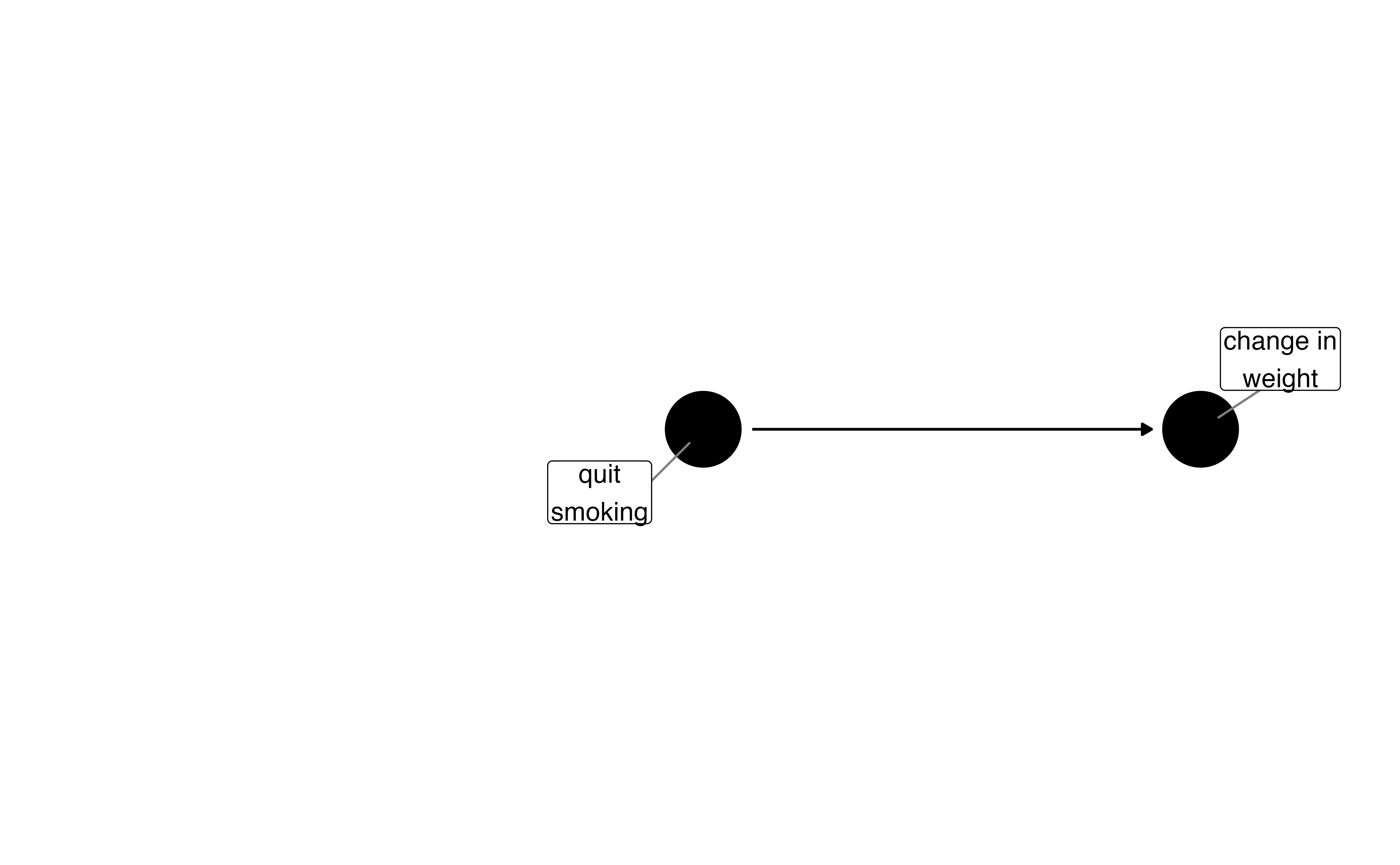
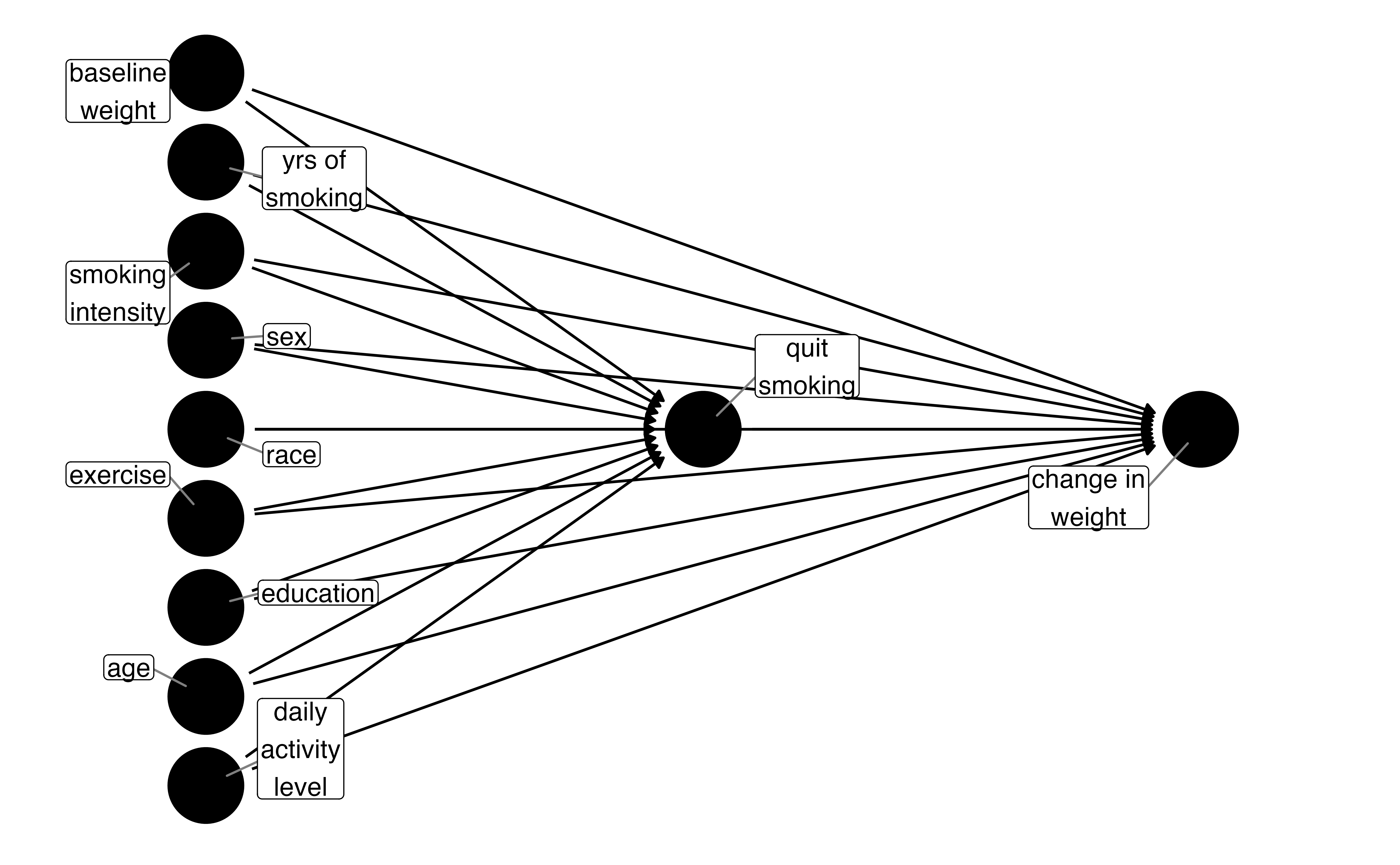
What do I need to control for?

Multivariable regression: what’s the association?

lm( 
  wt82_71~ qsmk + sex +  
    race + age + I(age^2) + education + 
    smokeintensity + I(smokeintensity^2) + 
    smokeyrs + I(smokeyrs^2) + exercise + active + 
    wt71 + I(wt71^2), 
  data = nhefs_complete_uc 
) |>
  tidy(conf.int = TRUE) |>
  filter(term == "qsmk")

# A tibble: 1 × 7
  term  estimate std.error statistic  p.value conf.low
  <chr>    <dbl>     <dbl>     <dbl>    <dbl>    <dbl>
1 qsmk      3.46     0.438      7.90 5.36e-15     2.60
# ℹ 1 more variable: conf.high <dbl>

model your assumptions

counterfactual: what if everyone quit smoking vs. what if no one quit smoking

Fit propensity score model

propensity_model <- glm( 
  qsmk ~ sex +  
    race + age + I(age^2) + education + 
    smokeintensity + I(smokeintensity^2) + 
    smokeyrs + I(smokeyrs^2) + exercise + active + 
    wt71 + I(wt71^2), 
  family = binomial(), 
  data = nhefs_complete_uc
)

Calculate inverse probability weights

library(propensity)
nhefs_complete_uc <- propensity_model |>
  # predict whether quit smoking
  augment(type.predict = "response", data = nhefs_complete_uc) |>
  # calculate inverse probability
  mutate(wts = wt_ate(.fitted, qsmk)) 

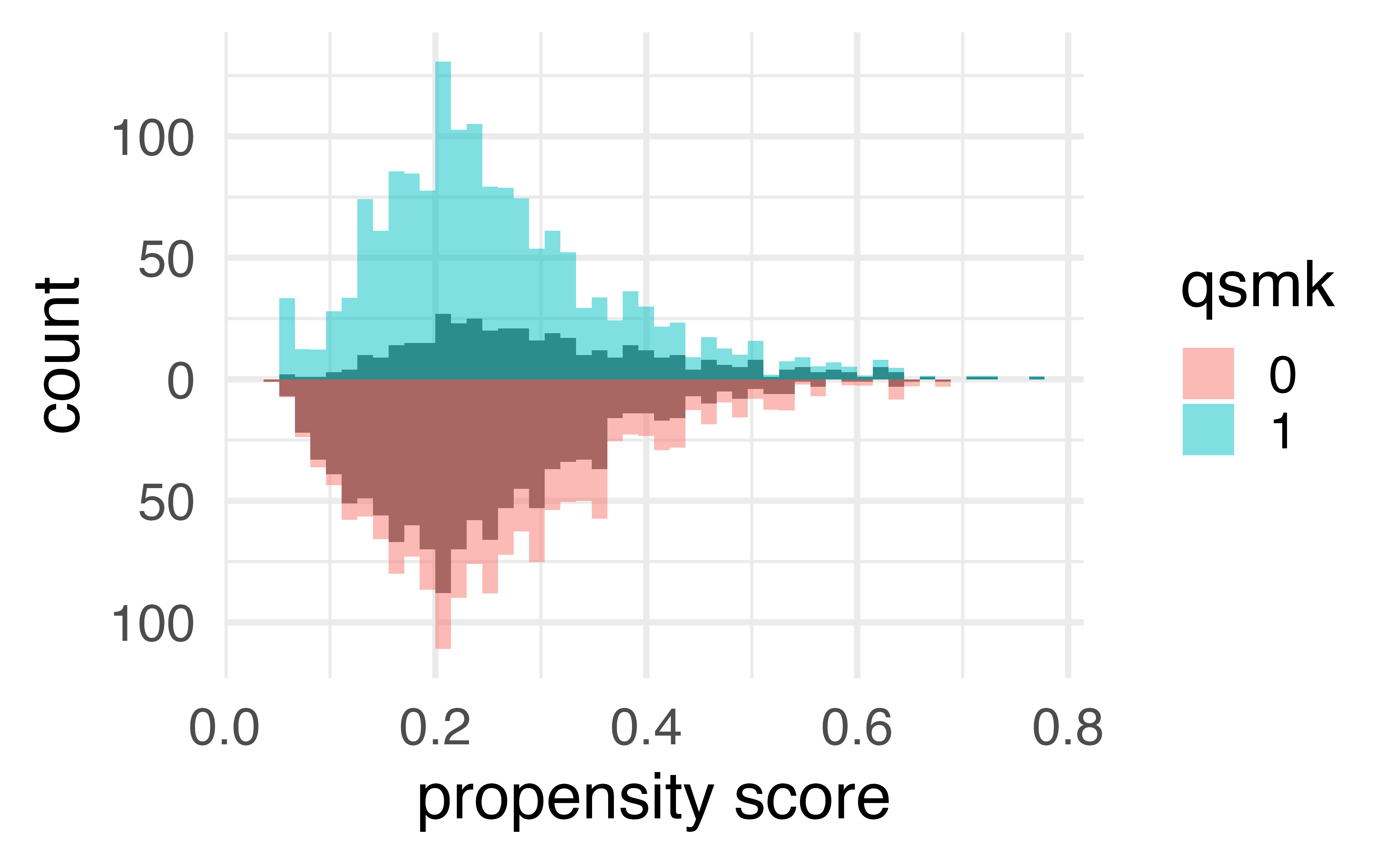
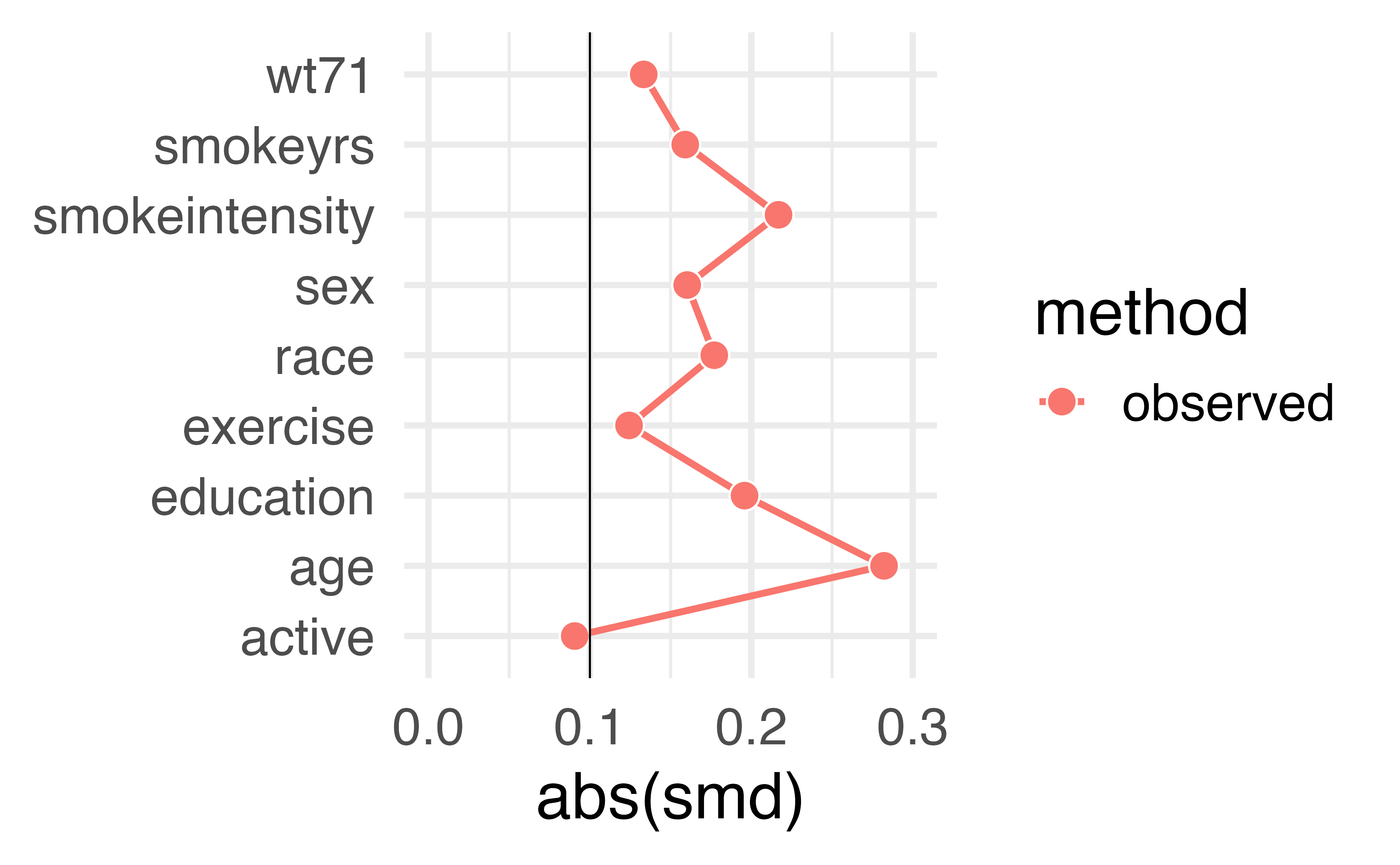
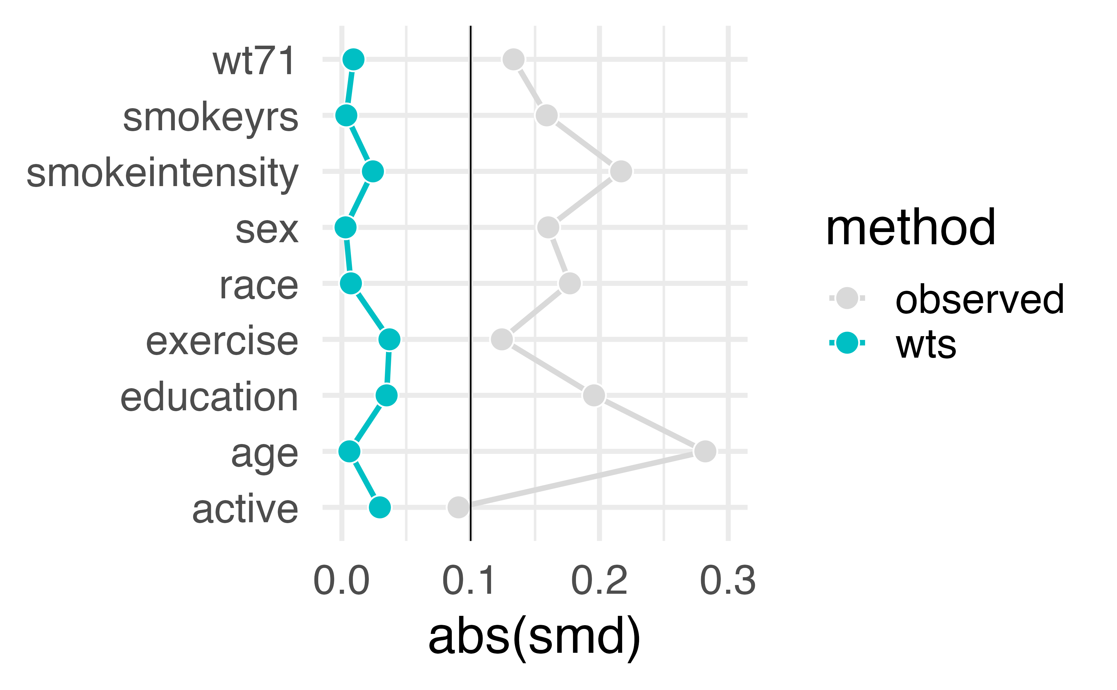
diagnose your model assumptions

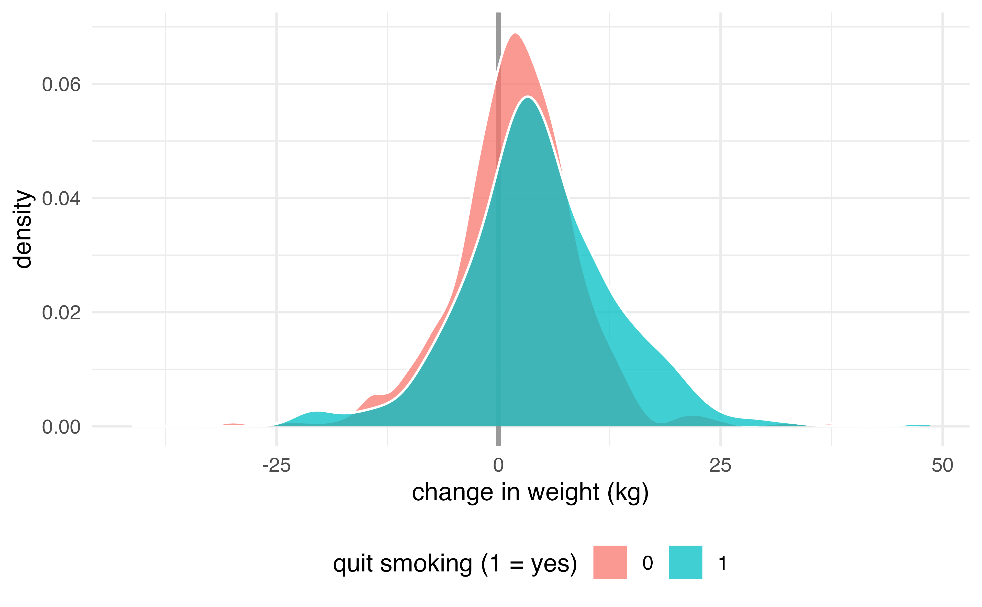
What’s the distribution of weights?

What are the weights doing to the sample?

What are the weights doing to the sample?

estimate the causal effects

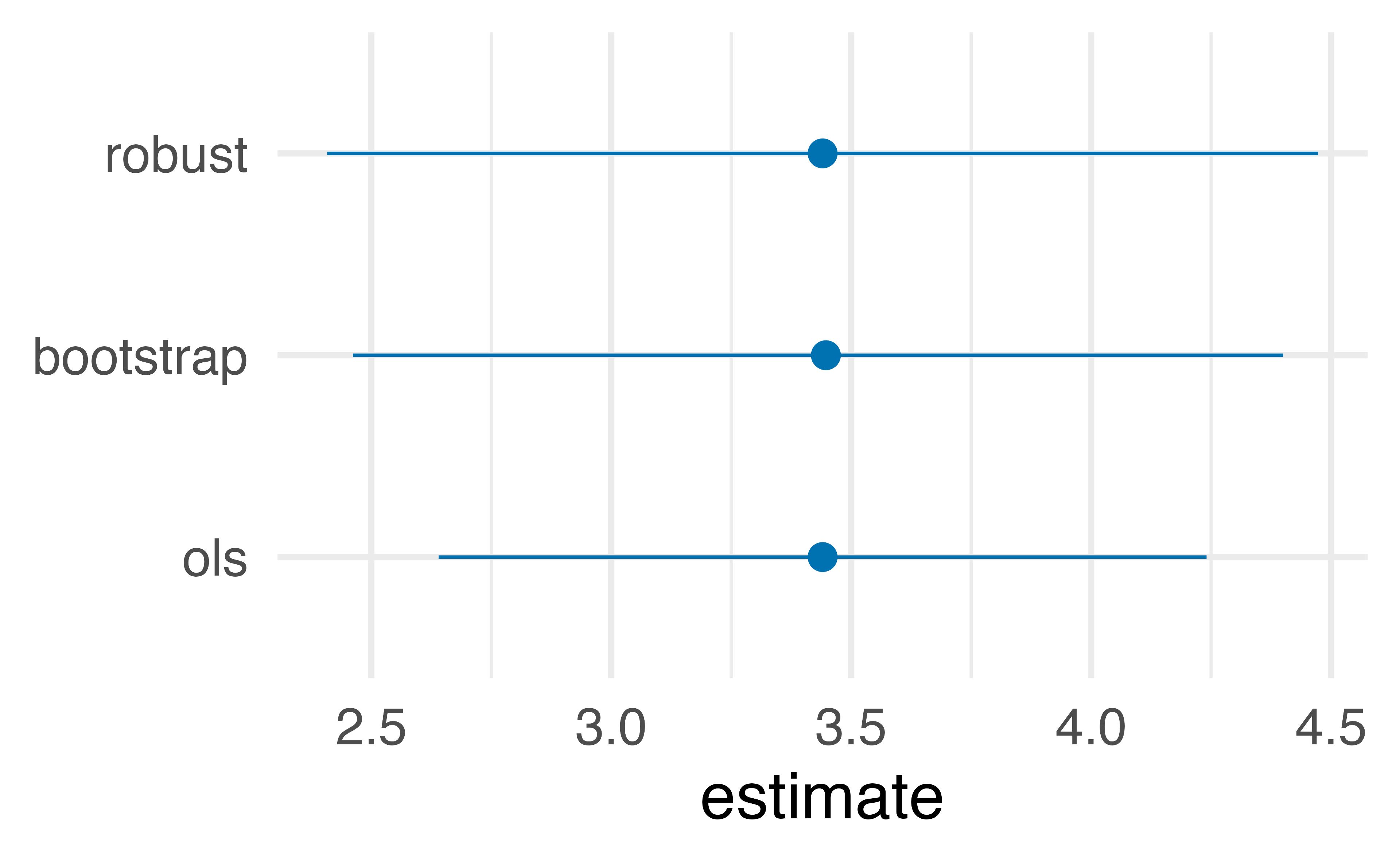
Estimate causal effect with IPW

ipw_model <- lm( 
  wt82_71 ~ qsmk, 
  data = nhefs_complete_uc, 
  weights = wts 
) 

ipw_estimate <- ipw_model |>
  tidy(conf.int = TRUE) |>
  filter(term == "qsmk")

Estimate causal effect with IPW

ipw_estimate

# A tibble: 1 × 7
  term  estimate std.error statistic  p.value conf.low
  <chr>    <dbl>     <dbl>     <dbl>    <dbl>    <dbl>
1 qsmk      3.44     0.408      8.43 7.47e-17     2.64
# ℹ 1 more variable: conf.high <dbl>

Let’s fix our confidence intervals with robust SEs!

# also see robustbase, survey, gee, and others
library(estimatr)
ipw_model_robust <- lm_robust( 
  wt82_71 ~ qsmk, 
  data = nhefs_complete_uc, 
  weights = wts 
) 

ipw_estimate_robust <- ipw_model_robust |>
  tidy(conf.int = TRUE) |>
  filter(term == "qsmk")

Let’s fix our confidence intervals with robust SEs!

as_tibble(ipw_estimate_robust)

# A tibble: 1 × 9
  term  estimate std.error statistic  p.value conf.low
  <chr>    <dbl>     <dbl>     <dbl>    <dbl>    <dbl>
1 qsmk      3.44     0.526      6.54 8.57e-11     2.41
# ℹ 3 more variables: conf.high <dbl>, df <dbl>,
#   outcome <chr>

Let’s fix our confidence intervals with the bootstrap!

# fit ipw model for a single bootstrap sample
fit_ipw_not_quite_rightly <- function(split, ...) { 
  # get bootstrapped data sample with `rsample::analysis()`
  .df <- analysis(split)
  
  # fit ipw model
  lm(wt82_71 ~ qsmk, data = .df, weights = wts) |>
    tidy()
}

fit_ipw <- function(split, ...) {
  .df <- analysis(split)
  
  # fit propensity score model
  propensity_model <- glm(
    qsmk ~ sex + 
      race + age + I(age^2) + education + 
      smokeintensity + I(smokeintensity^2) + 
      smokeyrs + I(smokeyrs^2) + exercise + active + 
      wt71 + I(wt71^2), 
    family = binomial(), 
    data = .df
  )
  
  # calculate inverse probability weights
  .df <- propensity_model |>
    augment(type.predict = "response", data = .df) |>
    mutate(wts = wt_ate(.fitted, qsmk))
  
  # fit correctly bootstrapped ipw model
  lm(wt82_71 ~ qsmk, data = .df, weights = wts) |>
    tidy()
}

Using {rsample} to bootstrap our causal effect

# fit ipw model to bootstrapped samples
ipw_results <- bootstraps(nhefs_complete_uc, 1000, apparent = TRUE) |>
  mutate(results = map(splits, fit_ipw)) 

Using {rsample} to bootstrap our causal effect

# get t-statistic-based CIs
boot_estimate <- int_t(ipw_results, results) |> 
  filter(term == "qsmk")

boot_estimate

Using {rsample} to bootstrap our causal effect

# A tibble: 1 × 6
  term  .lower .estimate .upper .alpha .method  
  <chr>  <dbl>     <dbl>  <dbl>  <dbl> <chr>    
1 qsmk    2.46      3.45   4.40   0.05 student-t

Our causal effect estimate: 3.5 kg (95% CI 2.4 kg, 4.4 kg)

Review the Quarto file… later!

Resources

Causal Inference: Comprehensive text on causal inference. Free online.

Bootstrap confidence intervals with {rsample}

R-causal: Our GitHub org with R packages and examples