When Standard Methods Succeed
Lucy D’Agostino McGowan
Wake Forest University
when correlation is causation
When you have no confounders and there is a linear relationship between the exposure and the outcome, that correlation is a causal relationship
😮
When you have no confounders and there is a linear relationship between the exposure and the outcome, that correlation is a causal relationship
😮
When you have no confounders and there is a linear relationship between the exposure and the outcome, that correlation is a causal relationship
😮
When you have no confounders and there is a linear relationship between the exposure and the outcome, that correlation is a causal relationship
😮
randomized controlled trials
A/B testing
Even in these cases, using the methods you will learn here can help!
- Adjusting for baseline covariates can make an estimate more efficient
- Propensity score weighting is more efficient than direct adjustment
- Sometimes we are more comfortable with the functional form of the propensity score (predicting exposure) than the outcome model
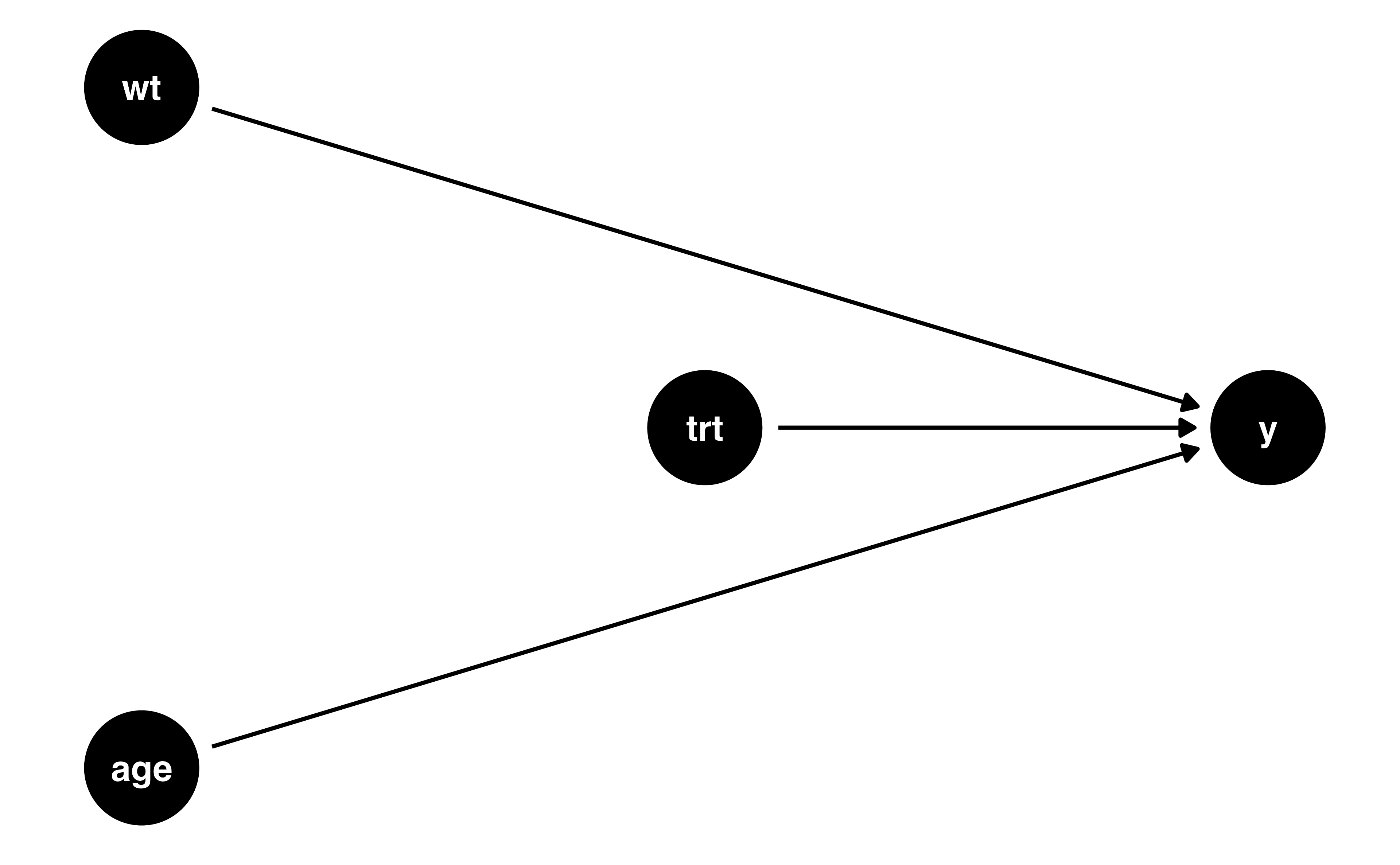
Example
- simulated data (100 observations)
- Treatment is randomly assigned
- There are two baseline covariates:
ageandweight
Example
- True average treatment effect: 1
Unadjusted model
| Characteristic | Beta | SE | 95% CI | p-value |
|---|---|---|---|---|
| treatment | 0.93 | 0.803 | -0.66, 2.5 | 0.2 |
| Abbreviations: CI = Confidence Interval, SE = Standard Error | ||||
Adjusted model
| Characteristic | Beta | SE | 95% CI | p-value |
|---|---|---|---|---|
| treatment | 1.0 | 0.204 | 0.59, 1.4 | <0.001 |
| weight | 0.34 | 0.106 | 0.13, 0.55 | 0.002 |
| age | 0.20 | 0.005 | 0.19, 0.22 | <0.001 |
| Abbreviations: CI = Confidence Interval, SE = Standard Error | ||||
Propensity score adjusted model
| Characteristic | Beta | SE | 95% CI | p-value |
|---|---|---|---|---|
| treatment | 1 | 0.202 | 0.6, 1.4 | <0.001 |
Example
- simulated data (10,000 observations)
- Treatment is randomly assigned
- There are two baseline covariates:
ageandweight
Unadjusted model
| Characteristic | Beta | SE | 95% CI | p-value |
|---|---|---|---|---|
| treatment | 0.96 | 0.083 | 0.80, 1.1 | <0.001 |
| Abbreviations: CI = Confidence Interval, SE = Standard Error | ||||
Adjusted model
| Characteristic | Beta | SE | 95% CI | p-value |
|---|---|---|---|---|
| treatment | 1.0 | 0.020 | 0.98, 1.1 | <0.001 |
| weight | 0.20 | 0.010 | 0.18, 0.22 | <0.001 |
| age | 0.20 | 0.000 | 0.20, 0.20 | <0.001 |
| Abbreviations: CI = Confidence Interval, SE = Standard Error | ||||
Propensity score adjusted model
| Characteristic | Beta | SE | 95% CI | p-value |
|---|---|---|---|---|
| treatment | 1 | 0.02 | 1, 1.1 | <0.001 |
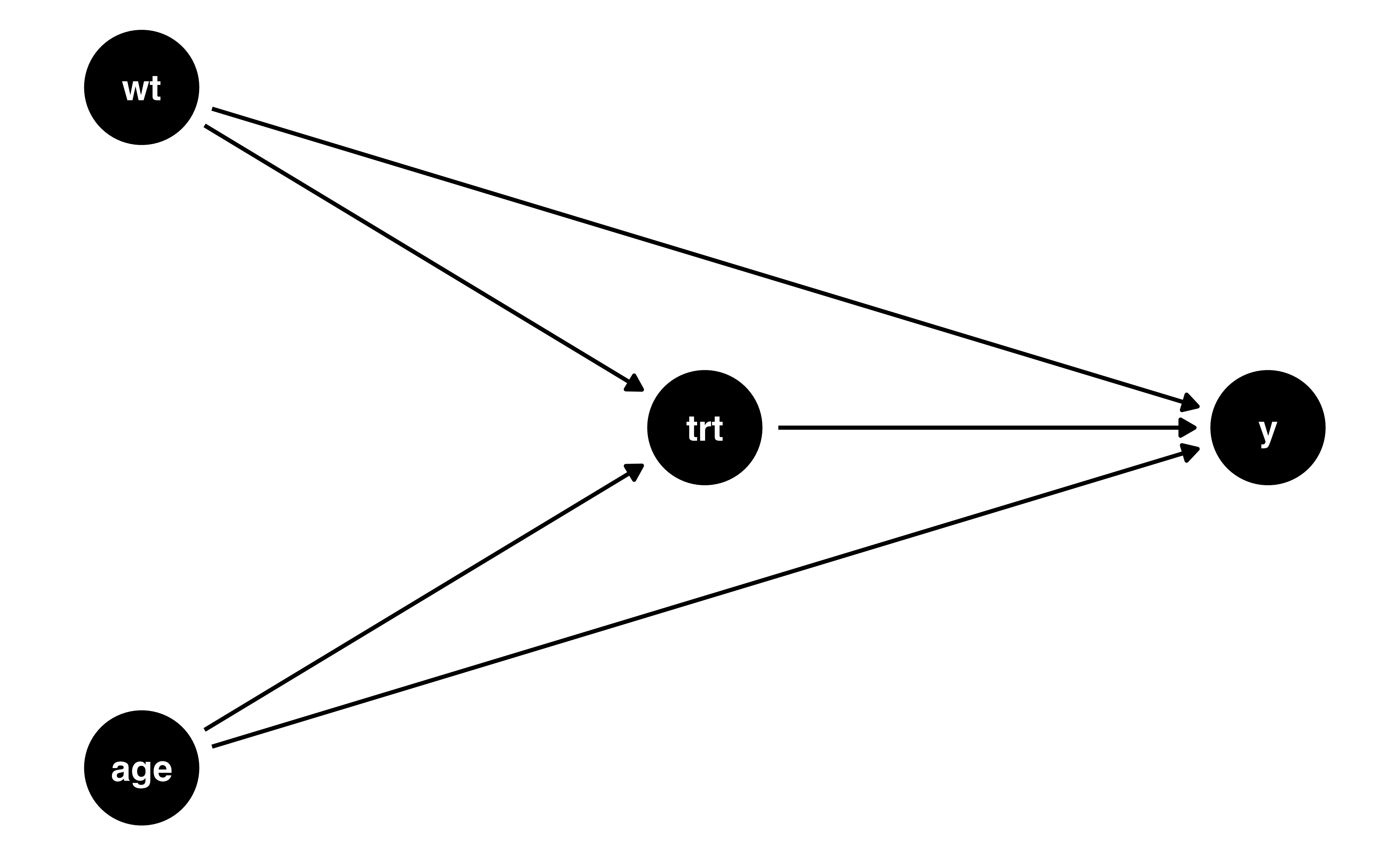
Example
- simulated data (10,000 observations)
- Treatment is not randomly assigned
- There are two baseline confounders:
ageandweight - The treatment effect is homogeneous
Example
- True average treatment effect: 1
Unadjusted model
| Characteristic | Beta | SE | 95% CI | p-value |
|---|---|---|---|---|
| treatment | 1.8 | 0.085 | 1.7, 2.0 | <0.001 |
| Abbreviations: CI = Confidence Interval, SE = Standard Error | ||||
Adjusted model
| Characteristic | Beta | SE | 95% CI | p-value |
|---|---|---|---|---|
| treatment | 0.98 | 0.021 | 0.94, 1.0 | <0.001 |
| weight | 0.20 | 0.010 | 0.18, 0.22 | <0.001 |
| age | 0.20 | 0.000 | 0.20, 0.20 | <0.001 |
| Abbreviations: CI = Confidence Interval, SE = Standard Error | ||||
Propensity score adjusted model
| Characteristic | Beta | SE | 95% CI | p-value |
|---|---|---|---|---|
| treatment | 1 | 0.022 | 0.9, 1 | <0.001 |