Causal Inference with `group_by` and `summarise`

Lucy D’Agostino McGowan

Wake Forest University

2022-07-23

Observational Studies

Goal: To answer a research question

Observational Studies

Goal: To answer a research question

Observational Studies

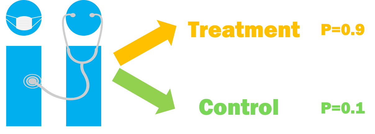
Randomized Controlled Trial

Observational Studies

Randomized Controlled Trial

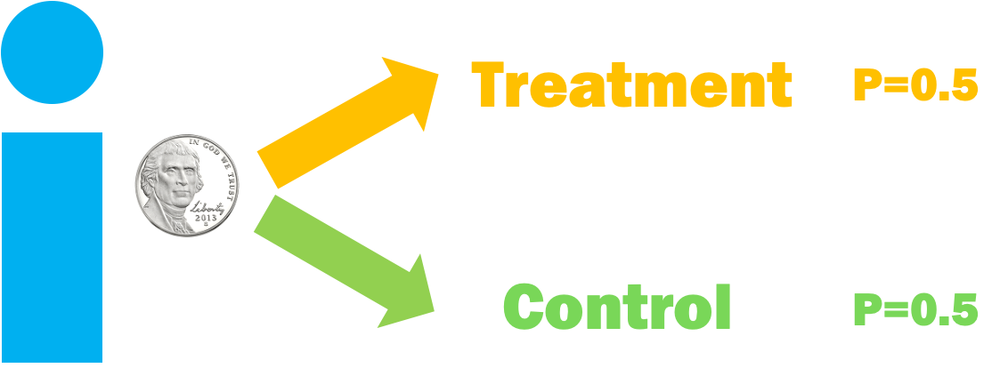
Observational Studies

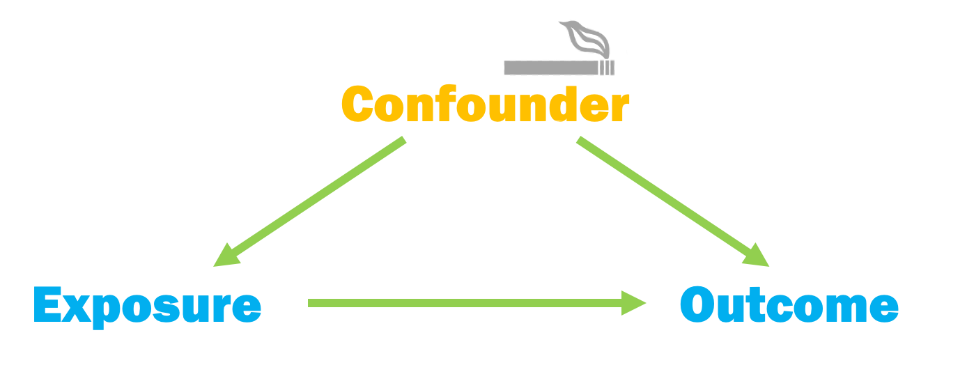
Confounding

One binary confounder

Simulation

n <- 1000 
sim <- tibble(
  confounder = rbinom(n, 1, 0.5),
  p_exposure = case_when(
    confounder == 1 ~ 0.75,
    confounder == 0 ~ 0.25
  ),
  exposure = rbinom(n, 1, p_exposure),
  outcome = confounder + rnorm(n)
)

# A tibble: 1,000 × 3
   confounder exposure outcome
        <int>    <int>   <dbl>
 1          0        0  1.13  
 2          0        0  1.11  
 3          1        1  0.129 
 4          1        0  1.21  
 5          0        0  0.0694
 6          1        1 -0.663 
 7          1        1  1.81  
 8          1        1 -0.912 
 9          1        0 -0.247 
10          0        0  0.998 
# ℹ 990 more rows

Simulation

lm(outcome ~ exposure, data = sim)


Call:
lm(formula = outcome ~ exposure, data = sim)

Coefficients:
(Intercept)     exposure  
     0.2688       0.4070

Simulation

sim |>
  group_by(exposure) |>
  summarise(avg_y = mean(outcome))

# A tibble: 2 × 2
  exposure avg_y
     <int> <dbl>
1        0 0.269
2        1 0.676

Simulation

sim |>
  group_by(exposure) |>
  summarise(avg_y = mean(outcome)) |>
  pivot_wider(
    names_from = exposure, 
    values_from = avg_y,  
    names_prefix = "x_"
  ) |>
  summarise(estimate = x_1 - x_0)

# A tibble: 1 × 1
  estimate
     <dbl>
1    0.407

Your Turn 1 (`03-ci-with-group-by-and-summarise-exercises.qmd`)

Group the dataset by `confounder` and `exposure`

Calculate the mean of the `outcome` for the groups

03:00

Your Turn 1

sim |>
  group_by(confounder, exposure) |>
  summarise(avg_y = mean(outcome))

# A tibble: 4 × 3
# Groups:   confounder [2]
  confounder exposure    avg_y
       <int>    <int>    <dbl>
1          0        0 -0.00907
2          0        1 -0.0166 
3          1        0  1.09   
4          1        1  0.936

Your Turn 1

sim |>
  group_by(confounder, exposure) |>
  summarise(avg_y = mean(outcome)) |>
  pivot_wider(
    names_from = exposure,
    values_from = avg_y,  
    names_prefix = "x_"
  ) |>
  summarise(estimate = x_1 - x_0) |>
  summarise(estimate = mean(estimate)) # note, we would need to weight this if the confounder groups were not equal sized

# A tibble: 1 × 1
  estimate
     <dbl>
1  -0.0794

🎉

Two binary confounders

Simulation

n <- 1000
sim2 <- tibble(
  confounder_1 = rbinom(n, 1, 0.5),
  confounder_2 = rbinom(n, 1, 0.5), 
  
  p_exposure = case_when(
    confounder_1 == 1 & confounder_2 == 1 ~ 0.75,
    confounder_1 == 0 & confounder_2 == 1 ~ 0.9,
    confounder_1 == 1 & confounder_2 == 0 ~ 0.2,
    confounder_1 == 0 & confounder_2 == 0 ~ 0.1,
  ),
  exposure = rbinom(n, 1, p_exposure),
  outcome = confounder_1 + confounder_2 + rnorm(n) 
)

# A tibble: 1,000 × 4
   confounder_1 confounder_2 exposure outcome
          <int>        <int>    <int>   <dbl>
 1            0            0        0   0.521
 2            1            0        0   1.38 
 3            0            0        0  -0.624
 4            0            1        1   0.427
 5            1            0        1   1.31 
 6            0            0        0  -0.707
 7            1            1        1   2.52 
 8            1            0        0   1.45 
 9            0            0        0  -0.505
10            0            1        1   0.793
# ℹ 990 more rows

Simulation

lm(outcome ~ exposure, data = sim2)


Call:
lm(formula = outcome ~ exposure, data = sim2)

Coefficients:
(Intercept)     exposure  
     0.6395       0.6951

Your Turn 2

Group the dataset by the confounders and exposure

Calculate the mean of the outcome for the groups

Your Turn 2

sim2 |>
  group_by(confounder_1, confounder_2, exposure) |>
  summarise(avg_y = mean(outcome)) |>
  pivot_wider(
    names_from = exposure,
    values_from = avg_y,  
    names_prefix = "x_"
  ) |>
  summarise(estimate = x_1 - x_0, .groups = "drop") |>
  summarise(estimate = mean(estimate))

# A tibble: 1 × 1
  estimate
     <dbl>
1  -0.0731

02:00

Simulation

n <- 100000 
big_sim2 <- tibble(
  confounder_1 = rbinom(n, 1, 0.5),
  confounder_2 = rbinom(n, 1, 0.5), 
  
  p_exposure = case_when(
    confounder_1 == 1 & confounder_2 == 1 ~ 0.75,
    confounder_1 == 0 & confounder_2 == 1 ~ 0.9,
    confounder_1 == 1 & confounder_2 == 0 ~ 0.2,
    confounder_1 == 0 & confounder_2 == 0 ~ 0.1,
  ),
  exposure = rbinom(n, 1, p_exposure),
  outcome = confounder_1 + confounder_2 + rnorm(n) 
)

# A tibble: 100,000 × 4
   confounder_1 confounder_2 exposure outcome
          <int>        <int>    <int>   <dbl>
 1            1            1        1   2.35 
 2            1            1        0   3.71 
 3            0            0        0   2.08 
 4            0            1        1   0.516
 5            0            0        0  -0.166
 6            1            1        1   1.58 
 7            0            0        0   0.472
 8            1            0        0   3.22 
 9            0            1        1   0.929
10            0            1        1   1.41 
# ℹ 99,990 more rows

Simulation

lm(outcome ~ exposure, data = big_sim2)


Call:
lm(formula = outcome ~ exposure, data = big_sim2)

Coefficients:
(Intercept)     exposure  
     0.6782       0.6561

Simulation

big_sim2 |>
  group_by(confounder_1, confounder_2, exposure) |>
  summarise(avg_y = mean(outcome)) |>
  pivot_wider(names_from = exposure,
              values_from = avg_y,  
              names_prefix = "x_") |>
  summarise(estimate = x_1 - x_0, .groups = "drop") |>
  summarise(estimate = mean(estimate))

# A tibble: 1 × 1
  estimate
     <dbl>
1   0.0187

Continuous confounder?

Simulation

n <- 10000 
sim3 <- tibble(
  confounder = rnorm(n), 
  p_exposure = exp(confounder) / (1 + exp(confounder)),
  exposure = rbinom(n, 1, p_exposure),
  outcome = confounder + rnorm(n) 
)

# A tibble: 10,000 × 3
   confounder exposure outcome
        <dbl>    <int>   <dbl>
 1     -0.167        0  -0.560
 2      0.252        1   0.628
 3     -0.321        1  -0.608
 4      0.621        0   1.58 
 5     -0.619        1   0.358
 6     -0.897        0  -1.95 
 7     -2.01         0  -2.50 
 8      0.296        0  -1.10 
 9     -0.504        1  -0.316
10     -0.536        1   1.12 
# ℹ 9,990 more rows

Simulation

lm(outcome ~ exposure, data = sim3)


Call:
lm(formula = outcome ~ exposure, data = sim3)

Coefficients:
(Intercept)     exposure  
    -0.4036       0.8152

Your Turn 3

Use `ntile()` from dplyr to calculate a binned version of `confounder` called `confounder_q`. We’ll create a variable with 5 bins.

Group the dataset by the binned variable you just created and exposure

Calculate the mean of the outcome for the groups

03:00

Your Turn 3

sim3 |>
  mutate(confounder_q = ntile(confounder, 5)) |>
  group_by(confounder_q, exposure) |>
  summarise(avg_y = mean(outcome)) |>
  pivot_wider(
    names_from = exposure,
    values_from = avg_y,  
    names_prefix = "x_"
  ) |>
  summarise(estimate = x_1 - x_0) |>
  summarise(estimate = mean(estimate))

# A tibble: 1 × 1
  estimate
     <dbl>
1   0.0728

Causal Inference with group_by and summarise

Observational Studies

Observational Studies

Observational Studies

Randomized Controlled Trial

Observational Studies

Randomized Controlled Trial

Observational Studies

Confounding

Confounding

One binary confounder

Simulation

Simulation

Simulation

Simulation

Your Turn 1 (03-ci-with-group-by-and-summarise-exercises.qmd)

Group the dataset by confounder and exposure

Calculate the mean of the outcome for the groups

Your Turn 1

Your Turn 1

Two binary confounders

Simulation

Simulation

Your Turn 2

Group the dataset by the confounders and exposure

Calculate the mean of the outcome for the groups

Your Turn 2

Simulation

Simulation

Simulation

Continuous confounder?

Simulation

Simulation

Your Turn 3

Use ntile() from dplyr to calculate a binned version of confounder called confounder_q. We’ll create a variable with 5 bins.

Group the dataset by the binned variable you just created and exposure

Calculate the mean of the outcome for the groups

Your Turn 3

What if we could come up with a summary score of all confounders?

Causal Inference with `group_by` and `summarise`

Your Turn 1 (`03-ci-with-group-by-and-summarise-exercises.qmd`)

Group the dataset by `confounder` and `exposure`

Calculate the mean of the `outcome` for the groups

Use `ntile()` from dplyr to calculate a binned version of `confounder` called `confounder_q`. We’ll create a variable with 5 bins.