Propensity Score Diagnostics
Lucy D’Agostino McGowan
Wake Forest University
Checking balance
- Love plots (Standardized Mean Difference)
- ECDF plots
Standardized Mean Difference (SMD)
\[\LARGE d = \frac{\bar{x}_{treatment}-\bar{x}_{control}}{\sqrt{\frac{s^2_{treatment}+s^2_{control}}{2}}}\]
SMD in R ![]()

Calculate standardized mean differences
Calculating SMDs
Calculating SMDs
# A tibble: 28 × 4
   variable       method   qsmk      smd
   <chr>          <chr>    <chr>   <dbl>
 1 sex1           observed 1      0.160
 2 race1          observed 1      0.177
 3 age            observed 1     -0.282
 4 education2     observed 1      0.112
 5 education3     observed 1      0.0472
 6 education4     observed 1      0.0270
 7 education5     observed 1     -0.166
 8 smokeintensity observed 1      0.217
 9 smokeyrs       observed 1     -0.159
10 exercise1      observed 1     -0.0398
# ℹ 18 more rows
Plotting SMDs ![]()
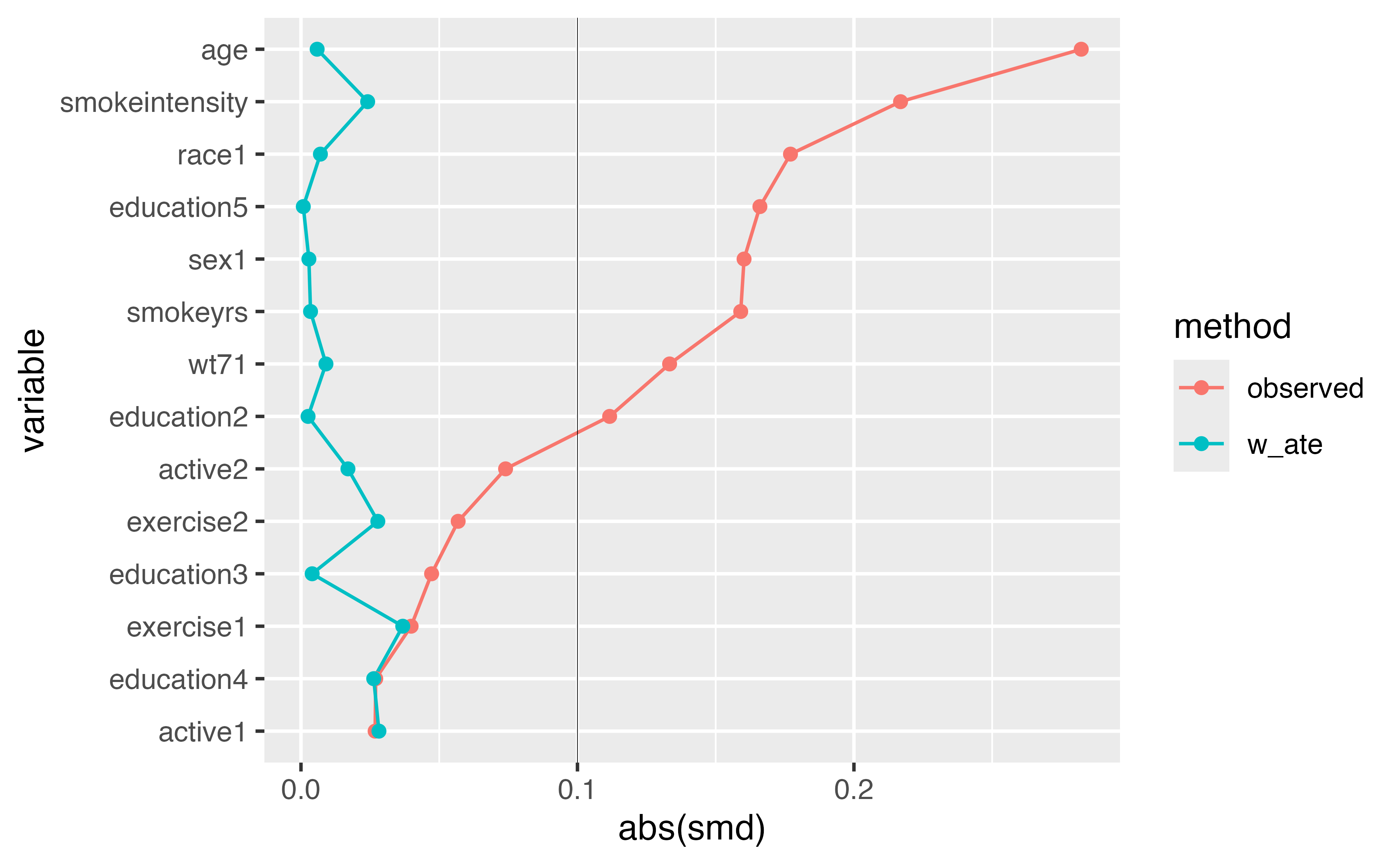
Plot them! (in a Love plot!)
Love plot
Your turn 1
06:00 Create a Love Plot for the propensity score weighting you created in the previous exercise
ECDF
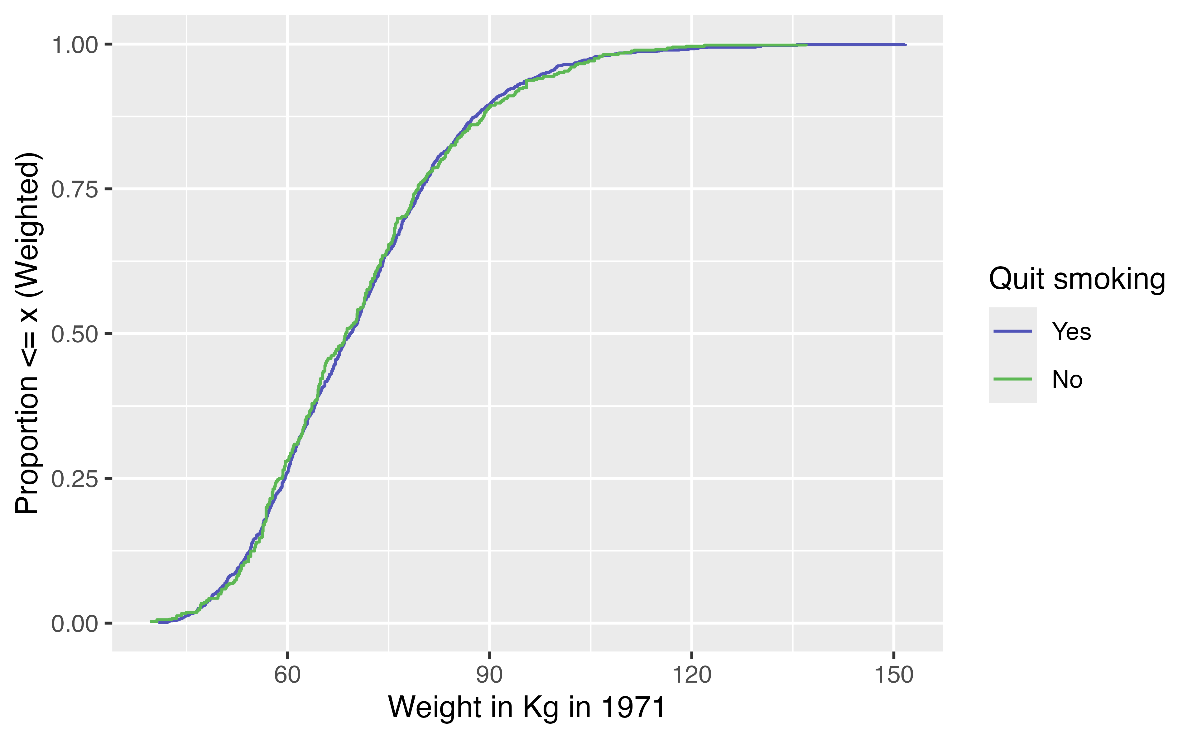
For continuous variables, it can be helpful to look at the whole distribution pre and post-weighting rather than a single summary measure
ECDF
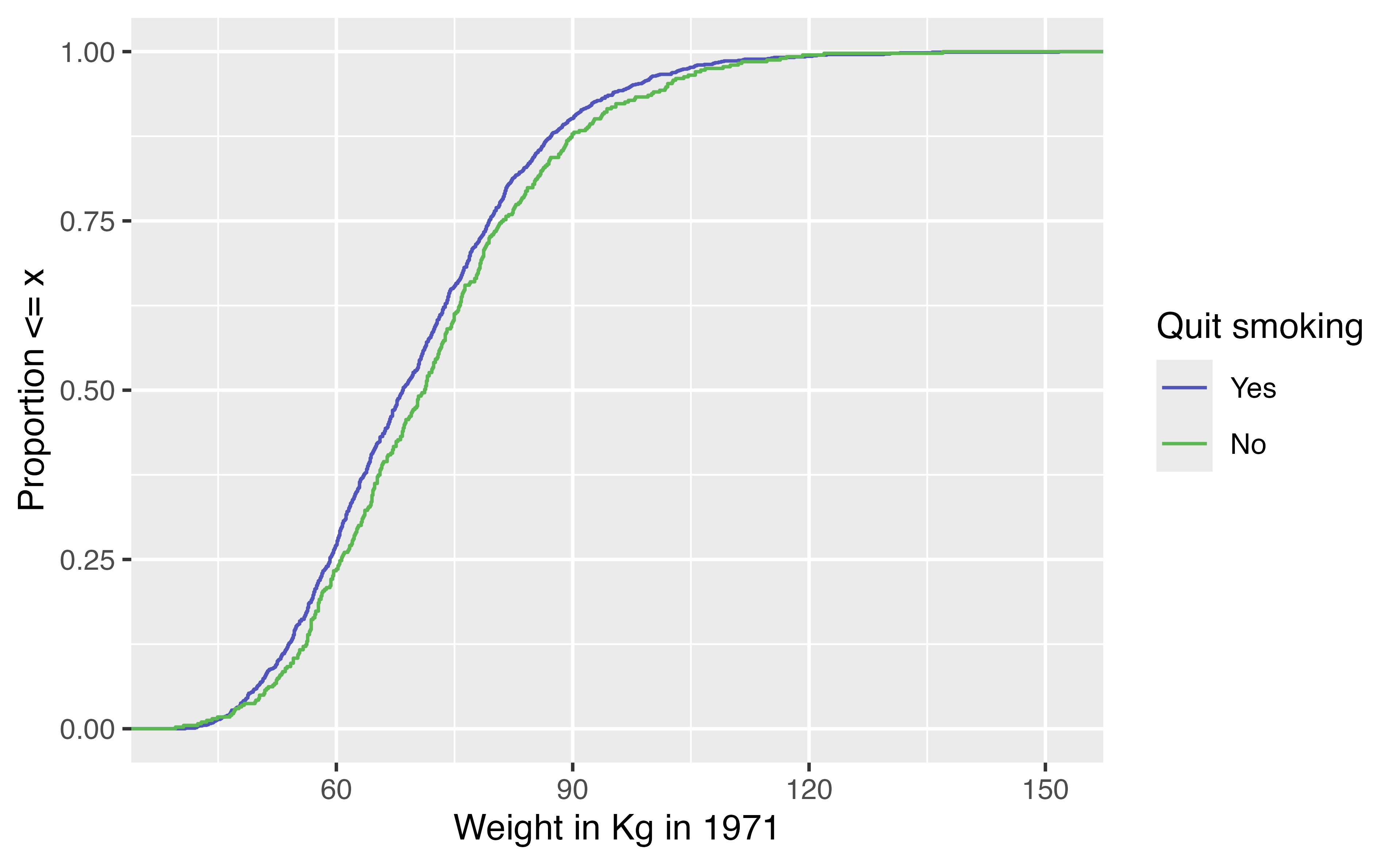
Unweighted ECDF
Unweighted ECDF

Weighted ECDF
Weighted ECDF
Your turn 2
06:00 Create an unweighted ECDF examining the park_temperature_high confounder by whether or not the day had Extra Magic Hours.
Create a weighted ECDF examining the park_temperature_high confounder
Bonus! Weighted Tables in R
1. Create a “design object” to incorporate the weights
2. Pass to gtsummary::tbl_svysummary()
| Characteristic | 0 N = 1,5651 |
1 N = 1,5611 |
Difference2 | 95% CI2 |
|---|---|---|---|---|
| WEIGHT IN KILOGRAMS IN 1971 | 69 (60, 80) | 69 (59, 79) | 0.01 | -0.06, 0.08 |
| 0: WHITE 1: BLACK OR OTHER IN 1971 | 0.01 | -0.06, 0.08 | ||
| 0 | 1,359 (87%) | 1,352 (87%) | ||
| 1 | 206 (13%) | 209 (13%) | ||
| AGE IN 1971 | 43 (33, 52) | 43 (33, 53) | -0.01 | -0.08, 0.06 |
| 0: MALE 1: FEMALE | 0.00 | -0.07, 0.07 | ||
| 0 | 764 (49%) | 764 (49%) | ||
| 1 | 802 (51%) | 797 (51%) | ||
| NUMBER OF CIGARETTES SMOKED PER DAY IN 1971 | 20 (10, 25) | 20 (10, 30) | 0.02 | -0.05, 0.09 |
| YEARS OF SMOKING | 24 (15, 33) | 24 (14, 33) | 0.00 | -0.07, 0.07 |
| IN RECREATION, HOW MUCH EXERCISE? IN 1971, 0:much exercise,1:moderate exercise,2:little or no exercise | 0.04 | -0.03, 0.11 | ||
| 0 | 302 (19%) | 294 (19%) | ||
| 1 | 665 (42%) | 691 (44%) | ||
| 2 | 599 (38%) | 576 (37%) | ||
| IN YOUR USUAL DAY, HOW ACTIVE ARE YOU? IN 1971, 0:very active, 1:moderately active, 2:inactive | 0.03 | -0.04, 0.10 | ||
| 0 | 700 (45%) | 684 (44%) | ||
| 1 | 718 (46%) | 738 (47%) | ||
| 2 | 147 (9.4%) | 138 (8.9%) | ||
| Abbreviation: CI = Confidence Interval | ||||
| 1 Median (Q1, Q3); n (%) | ||||
| 2 Standardized Mean Difference | ||||