Fitting the outcome model

Malcolm Barrett

2021-09-01

Outcome Model

library(broom)

lm(outcome ~ exposure, data = df, weights = wts) |>
  tidy()

✅ This will get us the point estimate

❌ This will get NOT us the correct confidence intervals

📦 {rsample}

1. Create a function to run your analysis once on a sample of your data

fit_ipw <- function(split, ...) {
  .df <- analysis(split)
  
  # fit propensity score model
  propensity_model <- glm(
    qsmk ~ sex + 
      race + age + I(age^2) + education + 
      smokeintensity + I(smokeintensity^2) + 
      smokeyrs + I(smokeyrs^2) + exercise + active + 
      wt71 + I(wt71^2), 
    family = binomial(), 
    data = .df
  )
  
  # calculate inverse probability weights
  .df <- propensity_model |>
    augment(type.predict = "response", data = .df) |>
    mutate(wts = wt_ate(.fitted, qsmk, exposure_type = "binary"))
  
  # fit correctly bootstrapped ipw model
  lm(wt82_71 ~ qsmk, data = .df, weights = wts) |>
    tidy()
}

2. Use {rsample} to bootstrap our causal effect

library(rsample)

# fit ipw model to bootstrapped samples
bootstrapped_nhefs <- bootstraps(
  nhefs_complete_uc, 
  times = 1000, 
  apparent = TRUE
)

bootstrapped_nhefs

2. Use {rsample} to bootstrap our causal effect

# Bootstrap sampling with apparent sample 
# A tibble: 1,001 × 2
   splits             id           
   <list>             <chr>        
 1 <split [1566/584]> Bootstrap0001
 2 <split [1566/580]> Bootstrap0002
 3 <split [1566/560]> Bootstrap0003
 4 <split [1566/595]> Bootstrap0004
 5 <split [1566/577]> Bootstrap0005
 6 <split [1566/544]> Bootstrap0006
 7 <split [1566/590]> Bootstrap0007
 8 <split [1566/572]> Bootstrap0008
 9 <split [1566/575]> Bootstrap0009
10 <split [1566/584]> Bootstrap0010
# ℹ 991 more rows

2. Use {rsample} to bootstrap our causal effect

fit_ipw(bootstrapped_nhefs$splits[[1]])

# A tibble: 2 × 5
  term        estimate std.error statistic  p.value
  <chr>          <dbl>     <dbl>     <dbl>    <dbl>
1 (Intercept)     1.54     0.294      5.26 1.65e- 7
2 qsmk            3.39     0.413      8.20 4.92e-16

2. Use {rsample} to bootstrap our causal effect

ipw_results <- bootstrapped_nhefs |> 
  mutate(boot_fits = map(splits, fit_ipw)) 

ipw_results

2. Use {rsample} to bootstrap our causal effect

# Bootstrap sampling with apparent sample 
# A tibble: 1,001 × 3
   splits             id            boot_fits       
   <list>             <chr>         <list>          
 1 <split [1566/587]> Bootstrap0001 <tibble [2 × 5]>
 2 <split [1566/555]> Bootstrap0002 <tibble [2 × 5]>
 3 <split [1566/590]> Bootstrap0003 <tibble [2 × 5]>
 4 <split [1566/599]> Bootstrap0004 <tibble [2 × 5]>
 5 <split [1566/580]> Bootstrap0005 <tibble [2 × 5]>
 6 <split [1566/574]> Bootstrap0006 <tibble [2 × 5]>
 7 <split [1566/572]> Bootstrap0007 <tibble [2 × 5]>
 8 <split [1566/569]> Bootstrap0008 <tibble [2 × 5]>
 9 <split [1566/562]> Bootstrap0009 <tibble [2 × 5]>
10 <split [1566/581]> Bootstrap0010 <tibble [2 × 5]>
# ℹ 991 more rows

2. Use {rsample} to bootstrap our causal effect

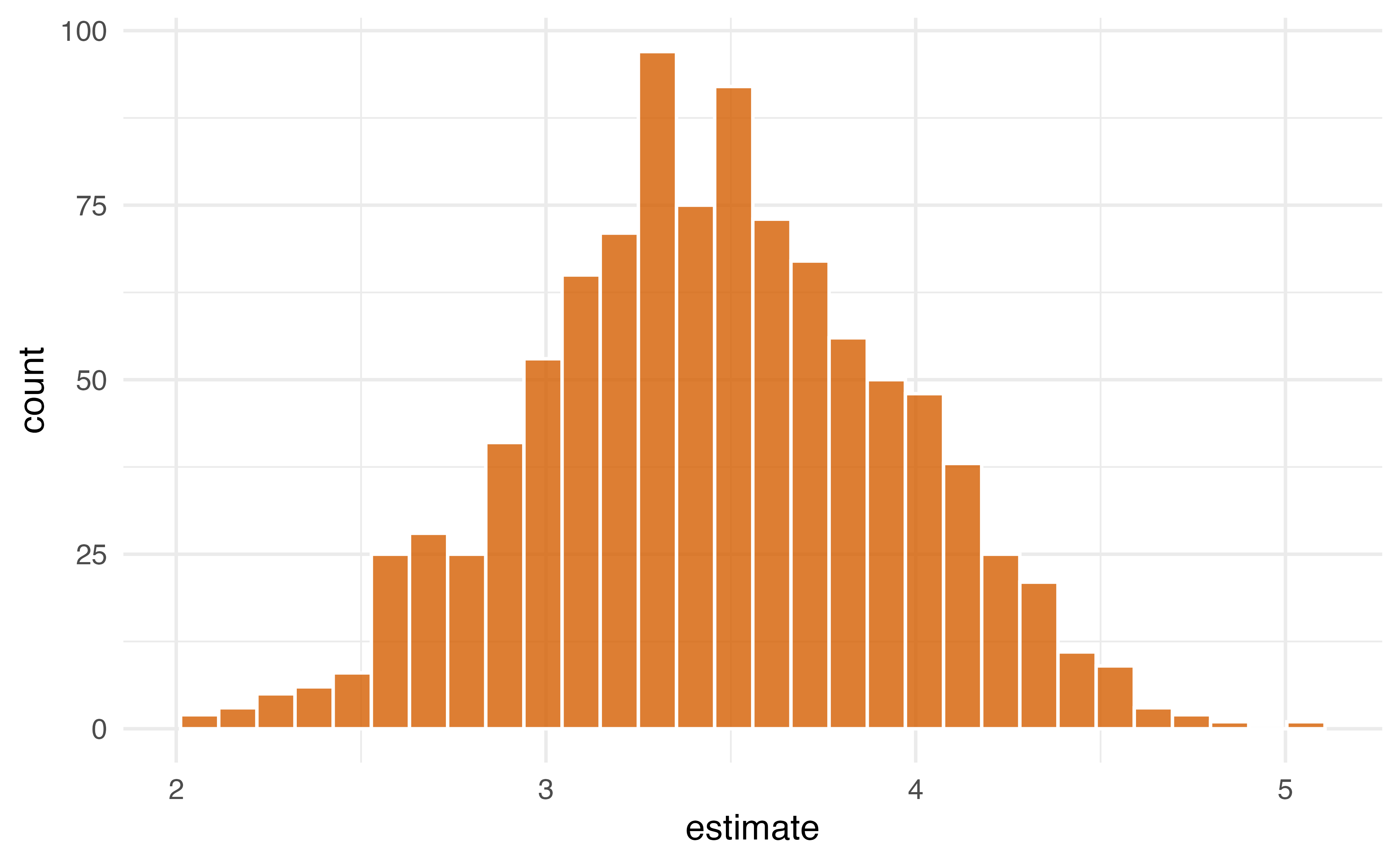
3. Pull out the causal effect

# get t-statistic-based CIs
boot_estimate <- int_t(ipw_results, boot_fits) |> 
  filter(term == "exposure")

Your Turn

12:00

Create a function called ipw_fit that fits the propensity score model and the weighted outcome model for the effect between park_extra_magic_morning and wait_minutes_posted_avg

Using the bootstraps() and int_t() functions to estimate the final effect.