Tipping Point Sensitivity Analyses

2021-09-01 (updated: 2023-08-31)

Lucy D’Agostino McGowan

Wake Forest University

Recall: Propensity scores

Rosenbaum and Rubin showed in observational studies, conditioning on propensity scores can lead to unbiased estimates of the exposure effect

There are no unmeasured confounders
Every subject has a nonzero probability of receiving either exposure

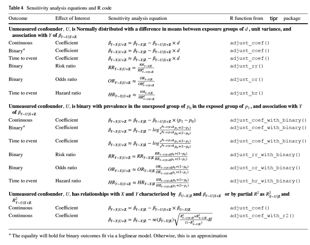
Quantifying Unmeasured Confounding

The exposure-outcome
The exposure-unmeasured
The unmeasured confounder-outcome effect

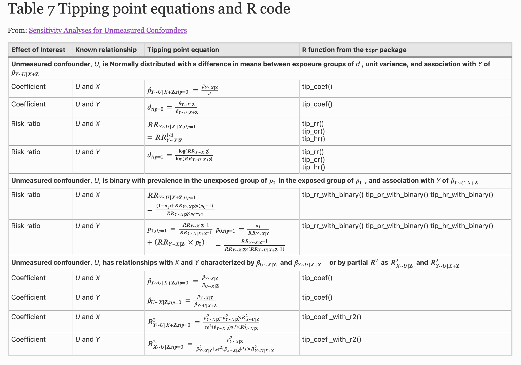
Quantifying Unmeasured Confounding

D’Agostino McGowan, L. Sensitivity Analyses for Unmeasured Confounders. Curr Epidemiol Rep 9, 361–375 (2022)

What will tip our confidence bound to cross zero?

Quantifying Unmeasured Confounding

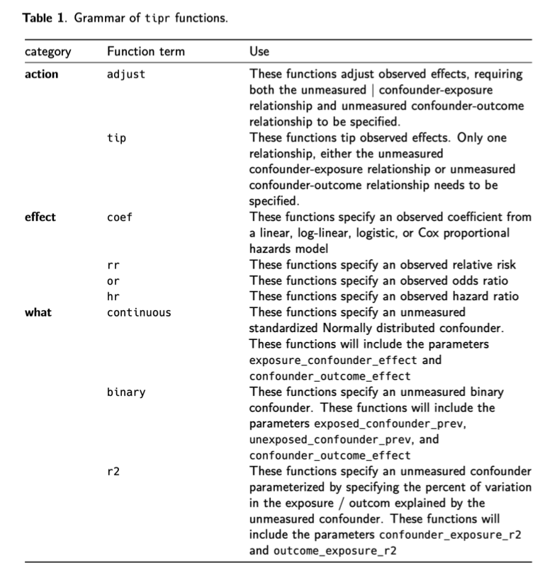
D’Agostino McGowan, L. Sensitivity Analyses for Unmeasured Confounders. Curr Epidemiol Rep 9, 361–375 (2022)

{action}_{effect}_with_{what}
tip_rr_with_continous()
adjust_coef_with_r2()

D’Agostino McGowan, L., (2022). tipr: An R package for sensitivity analyses for unmeasured confounders. Journal of Open Source Software, 7(77), 4495

tipr

Question

Analysis

New-user design
Matched 42,217 new metformin users to 42,217 new sulfonylurea users
Fit adjusted Cox proportional hazards model on the matched cohort

Results

Outcome: Lung Cancer
Adjusted Hazard Ratio: 0.87 (0.79, 0.96)

What if alcohol consumption is an unmeasured confounder?

What if heavy alcohol consumption is prevalent among 4% of Metformin users and 6% of Sulfonylurea users?

Meadows SO, Engel CC, Collins RL, Beckman RL, Cefalu M, Hawes-Dawson J, et al. 2015 health related behaviors survey: Substance use among US active-duty service members. RAND; 2018.

`tipr` Example

What if we assume the effect of alcohol consumption on lung cancer after adjusting for other confounders is 2?

library(tipr)
adjust_hr_with_binary(
  effect_observed = c(0.79, 0.87, 0.96),
  exposed_confounder_prev = .04,
  unexposed_confounder_prev = .06,
  confounder_outcome_effect = 2)

`tipr` Example

What if we assume the effect of alcohol consumption on lung cancer after adjusting for other confounders is 2?

library(tipr)
adjust_hr_with_binary(
  effect_observed = c(0.79, 0.87, 0.96),
  exposed_confounder_prev = .04,
  unexposed_confounder_prev = .06,
  confounder_outcome_effect = 2)

Results

Outcome: Lung Cancer
Adjusted Hazard Ratio: 0.87 (0.79, 0.96)

`tipr` Example

What if we assume the effect of alcohol consumption on lung cancer after adjusting for other confounders is 2?

library(tipr)
adjust_hr_with_binary(
  effect_observed = c(0.79, 0.87, 0.96),
  exposed_confounder_prev = .04,
  unexposed_confounder_prev = .06,
  confounder_outcome_effect = 2)

What if heavy alcohol consumption is prevalent among 4% of Metformin users and 6% of Sulfonylurea users?

Meadows SO, Engel CC, Collins RL, Beckman RL, Cefalu M, Hawes-Dawson J, et al. 2015 health related behaviors survey: Substance use among US active-duty service members. RAND; 2018.

`tipr` Example

What if we assume the effect of alcohol consumption on lung cancer after adjusting for other confounders is 2?

library(tipr)
adjust_hr_with_binary(
  effect_observed = c(0.79, 0.87, 0.96),
  exposed_confounder_prev = .04,
  unexposed_confounder_prev = .06,
  confounder_outcome_effect = 2)

`tipr` Example

# A tibble: 3 × 5
  hr_adjusted hr_observed exposed_confounder_prev unexposed_confounder_prev
        <dbl>       <dbl>                   <dbl>                     <dbl>
1       0.805        0.79                    0.04                      0.06
2       0.887        0.87                    0.04                      0.06
3       0.978        0.96                    0.04                      0.06
# ℹ 1 more variable: confounder_outcome_effect <dbl>

“If heavy alcohol consumption differed between groups, with 4% prevalence among metformin users and 6% among sulfonylureas users, and had an HR of 2 with lung cancer incidence the updated adjusted effect of metformin on lung cancer incidence would be an HR of 0.89 (95% CI: 0.81–0.98). Should an unmeasured confounder like this exist, our effect of metformin on lung cancer incidence would be attenuated and fall much closer to the null.

`tipr` Example

library(tipr)
sens <- adjust_hr_with_binary(
  effect_observed = 0.96,
  exposed_confounder_prev = .04,
  unexposed_confounder_prev = .06,
  confounder_outcome_effect = seq(1.1, 3.5, by = 0.1))

`tipr` Example

library(ggplot2)
ggplot(sens, aes(x = confounder_outcome_effect, y = hr_adjusted)) + 
  geom_point() +
  geom_hline(yintercept = 1, lty = 2)

`tipr` Example

library(tipr)
tip_hr_with_binary(
  effect_observed = 0.96,
  exposed_confounder_prev = .04,
  unexposed_confounder_prev = .06)

`tipr` Example

# A tibble: 1 × 6
  effect_adjusted effect_observed exposed_confounder_prev unexposed_confounder…¹
            <dbl>           <dbl>                   <dbl>                  <dbl>
1               1            0.96                    0.04                   0.06
# ℹ abbreviated name: ¹unexposed_confounder_prev
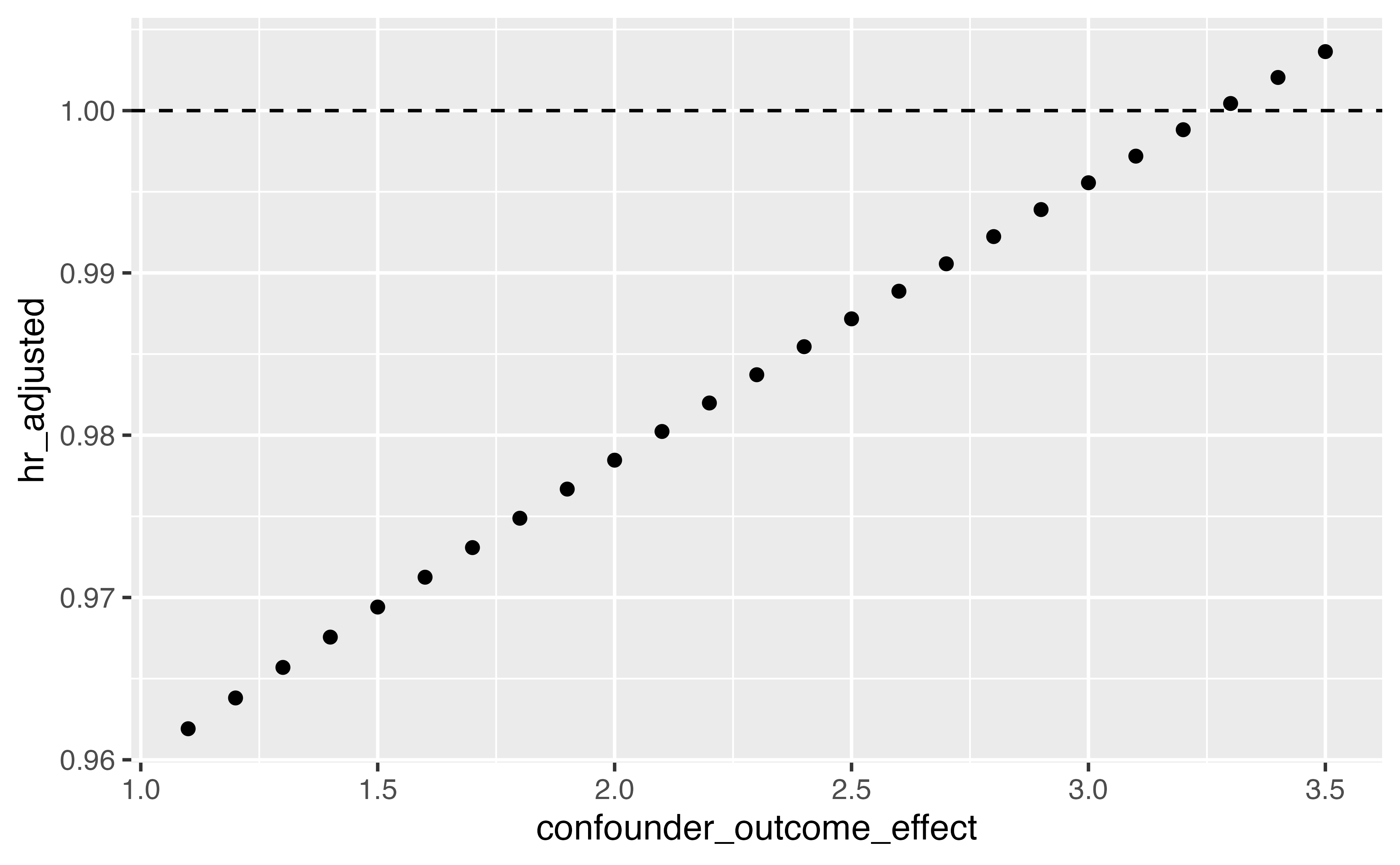
# ℹ 2 more variables: confounder_outcome_effect <dbl>,
#   n_unmeasured_confounders <dbl>

“If heavy alcohol consumption differed between groups, with 4% prevalence among metformin users and 6% among sulfonylureas users, it would need to have an association with lung cancer incidence of 3.27 to tip this analysis at the 5% level, rendering it inconclusive. This effect is larger than the understood association between lung cancer and alcohol consumption.”

What is known about the unmeasured confounder?

Both exposure and outcome relationship is known

adjust_* functions

Only one of the exposure/outcome relationships is known

adjust_* functions in an array
tip_* functions

Nothing is known

adjust_* functions in an array
tip_* functions in an array
tip_coef_with_r2() (measured confounders)
Robustness value r_value() & E-values e_value()

Disney Data

`tip_coef()`

effect_observed: observed exposure - outcome effect 4.32 minutes (95% CI: 0.0009, 8.36)

Disney Data

`tip_coef()`

exposure_confounder_effect: scaled mean difference between the unmeasured confounder in the exposed and unexposed population

Disney Data

`tip_coef()`

confounder_outcome_effect: relationship between the unmeasured confounder and outcome

Your turn

05:00

Use the `tip_coef()` function to conduct a sensitivity analysis for the estimate from your previous exercises. Use the lower bound of the confidence interval for the effect and `0.1` for the exposure-confounder effect.

Tipping Point Sensitivity Analyses

Recall: Propensity scores

Quantifying Unmeasured Confounding

Quantifying Unmeasured Confounding

Quantifying Unmeasured Confounding

What will tip our confidence bound to cross zero?

Quantifying Unmeasured Confounding

tipr

Question

Analysis

Results

What if alcohol consumption is an unmeasured confounder?

What if heavy alcohol consumption is prevalent among 4% of Metformin users and 6% of Sulfonylurea users?

tipr Example

tipr Example

Results

tipr Example

What if heavy alcohol consumption is prevalent among 4% of Metformin users and 6% of Sulfonylurea users?

tipr Example

tipr Example

tipr Example

tipr Example

tipr Example

tipr Example

What is known about the unmeasured confounder?

Both exposure and outcome relationship is known

Only one of the exposure/outcome relationships is known

Nothing is known

Disney Data

tip_coef()

Disney Data

tip_coef()

Disney Data

tip_coef()

Your turn

Use the tip_coef() function to conduct a sensitivity analysis for the estimate from your previous exercises. Use the lower bound of the confidence interval for the effect and 0.1 for the exposure-confounder effect.

`tipr` Example

`tipr` Example

`tipr` Example

`tipr` Example

`tipr` Example

`tipr` Example

`tipr` Example

`tipr` Example

`tipr` Example

`tip_coef()`

`tip_coef()`

`tip_coef()`

Use the `tip_coef()` function to conduct a sensitivity analysis for the estimate from your previous exercises. Use the lower bound of the confidence interval for the effect and `0.1` for the exposure-confounder effect.