Bonus: Colliders, selection bias, and loss to follow-up
Malcolm Barrett
Stanford University
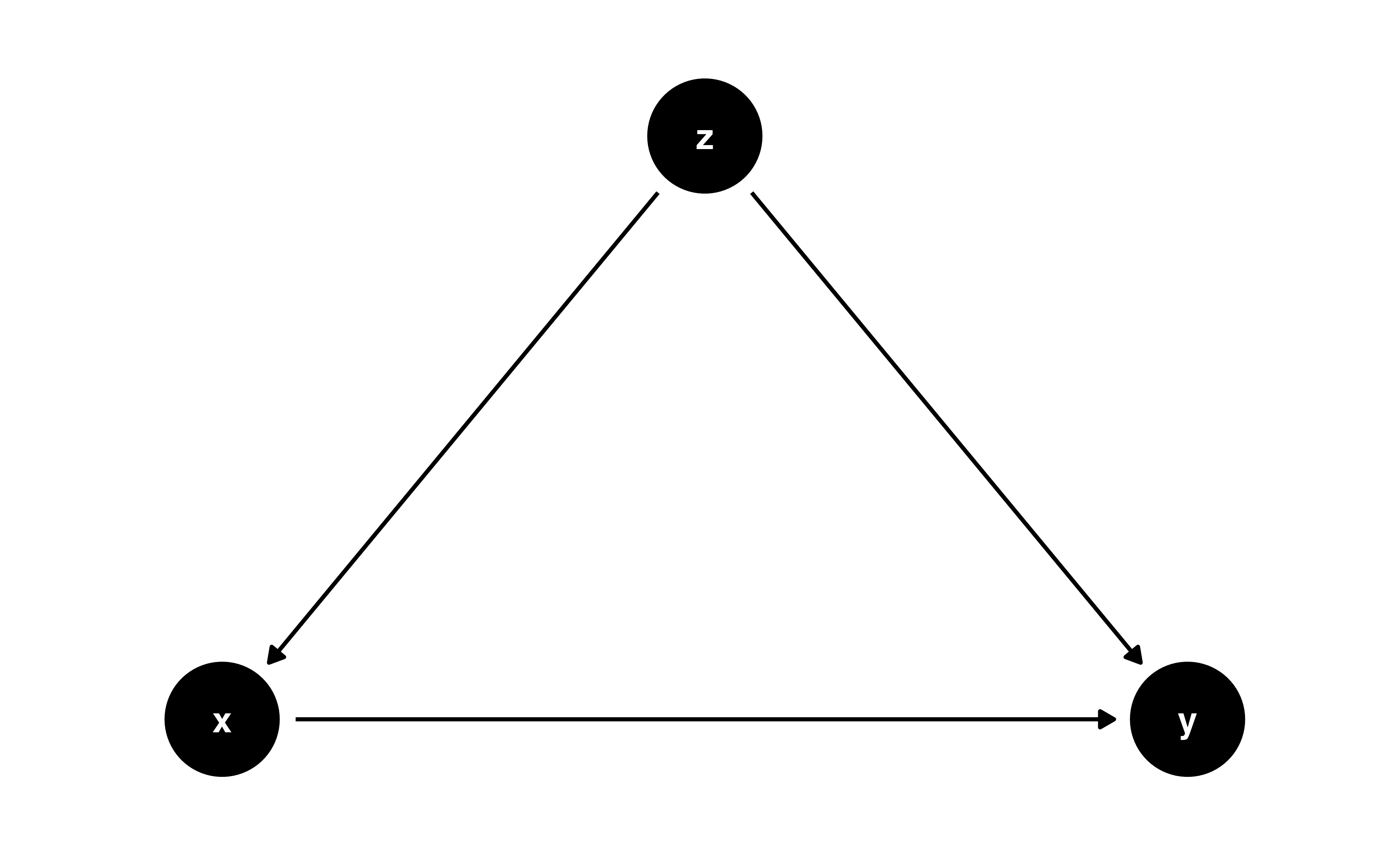
Confounders and chains

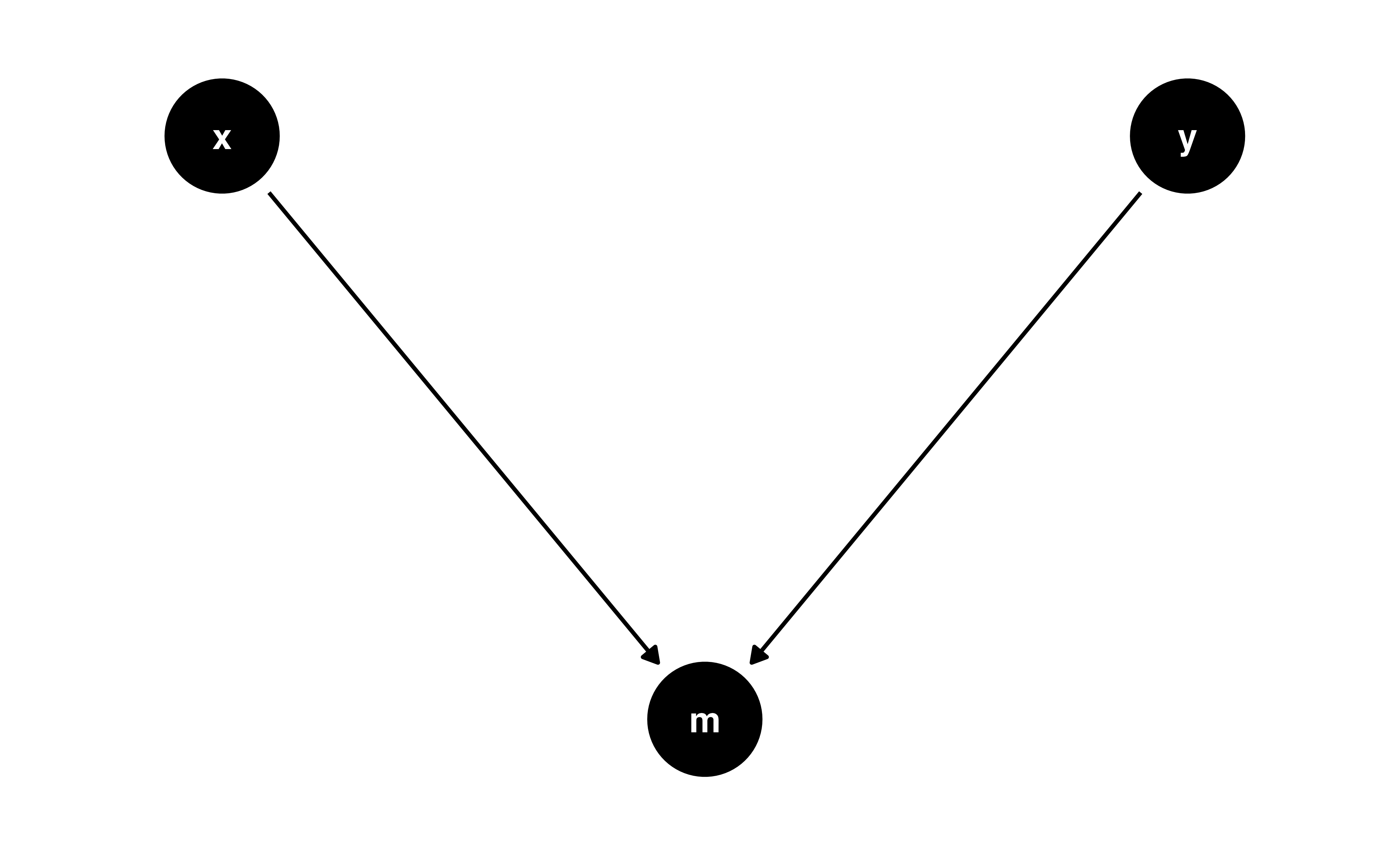
Colliders

Colliders

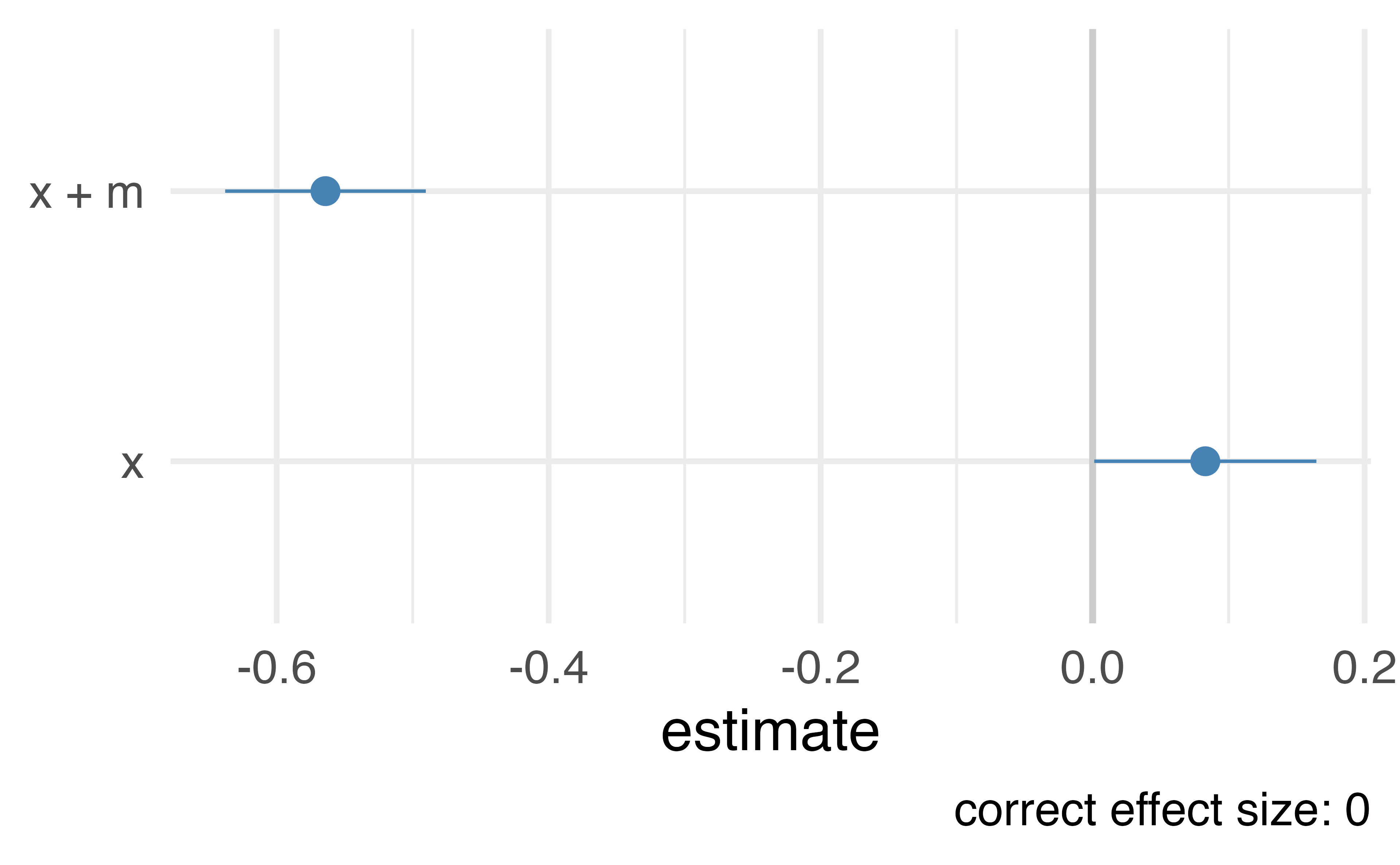
Let’s prove it!
Let’s prove it!
Let’s prove it!

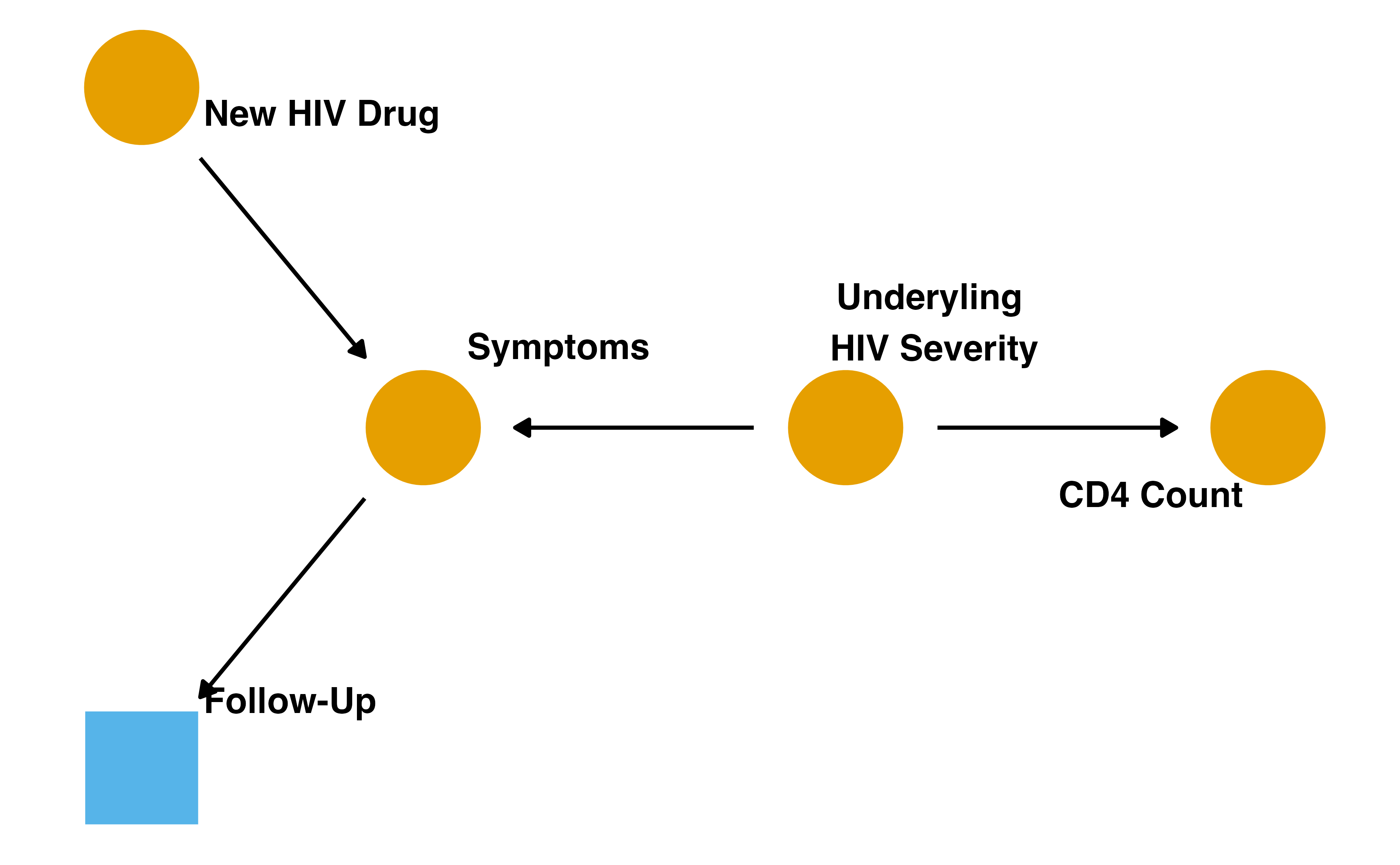
Loss to follow-up

Adjusting for selection bias
- Fit a probability of censoring model, e.g. glm(censoring ~ predictors, family = binomial())
- Create weights using inverse probability strategy
- Use weights in your causal model
We won’t do it here, but you can include many types of weights in a given model. Just take their product, e.g. multiply inverse propensity of treatment weights by inverse propensity of censoring weights.
Your Turn
Work through Your Turns 1-3 in 13-bonus-selection-bias.qmd
10:00