Continuous exposures with propensity scores

Malcolm Barrett

2021-09-01

Warning! Propensity score weights are sensitive to positivity violations for continuous exposures.

The story so far

Propensity score weighting

1. Fit a propensity model predicting exposure x, x + z where z is all covariates
2. Calculate weights
3. Fit an outcome model estimating the effect of x on y weighted by the propensity score

Continous exposures

1. Use a model like lm(x ~ z) for the propensity score model.
2. Use wt_ate() with .fitted and .sigma; transforms using dnorm() to get on probability-like scale.
3. Apply the weights to the outcome model as normal!

Alternative: quantile binning

1. Bin the continuous exposure into quantiles and use categorical regression like a multinomial model to calculate probabilities.
2. Calculate the weights where the propensity score is the probability you fall into the quantile you actually fell into. Same as the binary ATE!
3. Same workflow for the outcome model

1. Fit a model for exposure ~ confounders

model <- lm(
  exposure ~ confounder_1 + confounder_2,
  data = df
)

2. Calculate the weights with wt_ate()

model |>
  augment(data = df) |>
  mutate(wts = wt_ate( 
    exposure, 
    .fitted, 
    # .sigma is from augment()
    .sigma = .sigma
  )) 

Does change in smoking intensity (smkintensity82_71) affect weight gain among lighter smokers?

nhefs_light_smokers <- nhefs_complete |>
  filter(smokeintensity <= 25)

1. Fit a model for exposure ~ confounders

nhefs_model <- lm(
  smkintensity82_71 ~ sex + race + age + I(age^2) + 
    education + smokeintensity + I(smokeintensity^2) + 
    smokeyrs + I(smokeyrs^2) + exercise + active + 
    wt71 + I(wt71^2), 
  data = nhefs_light_smokers
)

2. Calculate the weights with wt_ate()

nhefs_wts <- nhefs_model |> 
  augment(data = nhefs_light_smokers) |> 
  mutate(wts = wt_ate(
    smkintensity82_71, 
    .fitted,
    .sigma = .sigma
  )) 

2. Calculate the weights with wt_ate()

nhefs_wts

# A tibble: 1,162 × 74
    seqn  qsmk death yrdth modth dadth   sbp   dbp sex  
   <dbl> <dbl> <dbl> <dbl> <dbl> <dbl> <dbl> <dbl> <fct>
 1   235     0     0    NA    NA    NA   123    80 0    
 2   244     0     0    NA    NA    NA   115    75 1    
 3   245     0     1    85     2    14   148    78 0    
 4   252     0     0    NA    NA    NA   118    77 0    
 5   257     0     0    NA    NA    NA   141    83 1    
 6   262     0     0    NA    NA    NA   132    69 1    
 7   266     0     0    NA    NA    NA   100    53 1    
 8   419     0     1    84    10    13   163    79 0    
 9   420     0     1    86    10    17   184   106 0    
10   434     0     0    NA    NA    NA   127    80 1    
# ℹ 1,152 more rows
# ℹ 65 more variables: age <dbl>, race <fct>, income <dbl>,
#   marital <dbl>, school <dbl>, education <fct>, …

Do posted wait times at 8 am affect actual wait times at 9 am?

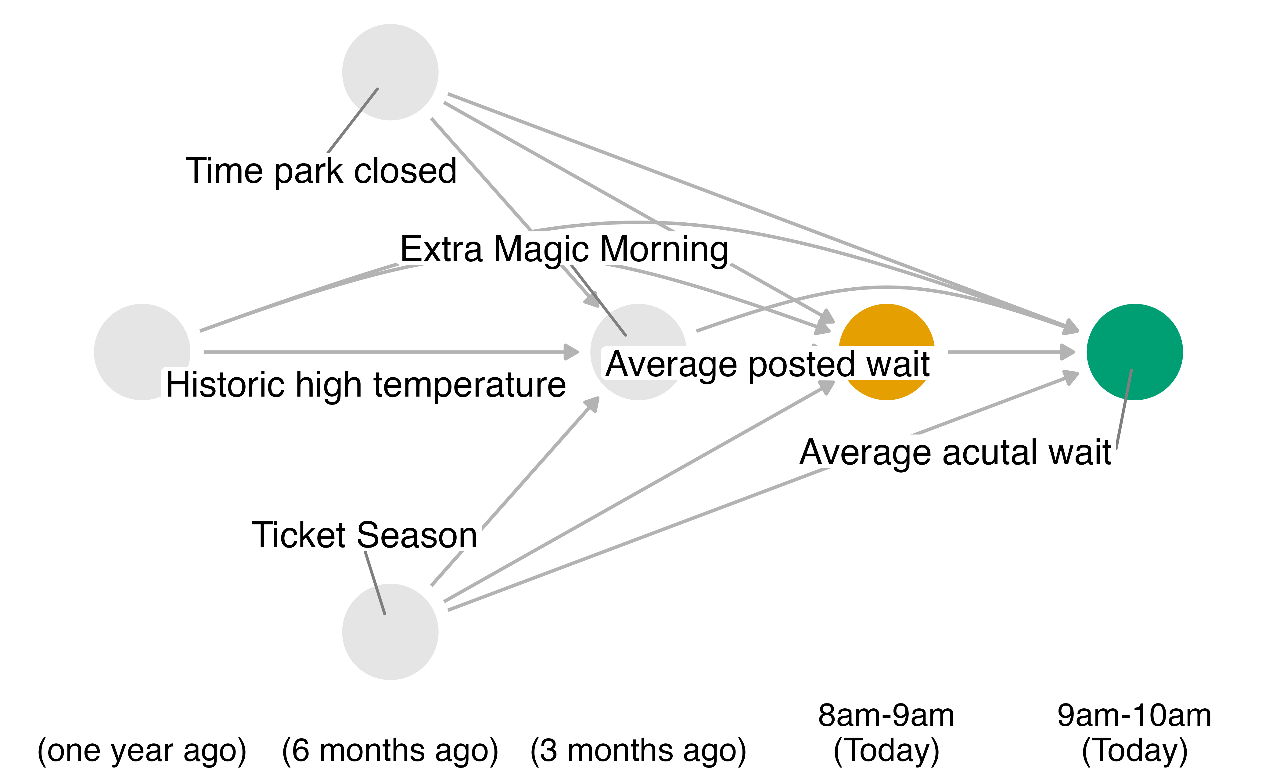
Your Turn 1

Fit a model using lm() with wait_minutes_posted_avg as the outcome and the confounders identified in the DAG.

Use augment() to add model predictions to the data frame

In wt_ate(), calculate the weights using wait_minutes_posted_avg, .fitted, and .sigma

05:00

Your Turn 1

post_time_model <- lm(
  wait_minutes_posted_avg ~
    park_close + park_extra_magic_morning + 
    park_temperature_high + park_ticket_season, 
  data = wait_times
)

Your Turn 1

wait_times_wts <- post_time_model |>
  augment(data = wait_times) |>
  mutate(wts = wt_ate(
    wait_minutes_posted_avg, .fitted, .sigma = .sigma
  ))

Stabilizing extreme weights

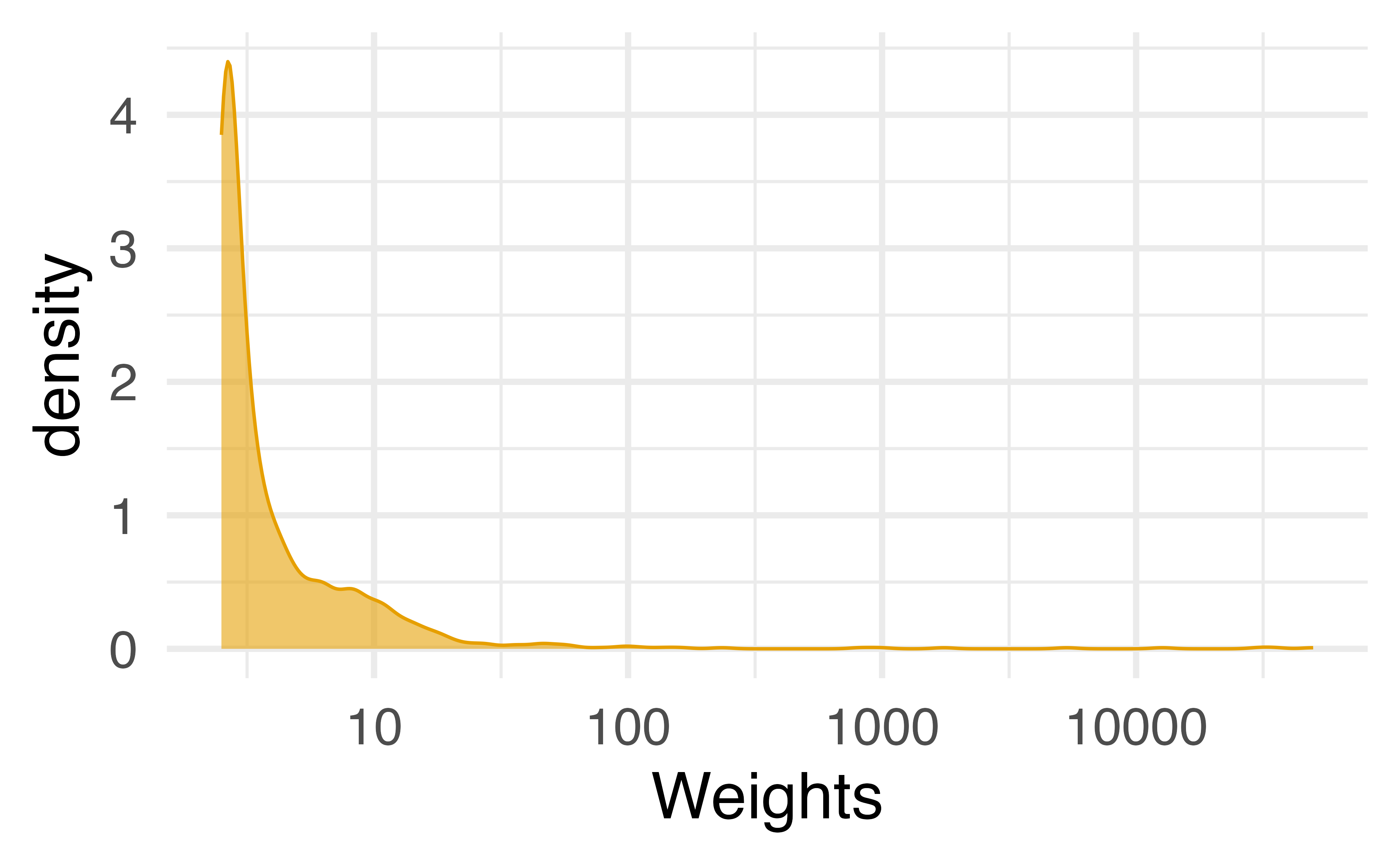
Stabilizing extreme weights

1. Fit an intercept-only model (e.g. lm(x ~ 1)) or use mean and SD of x
2. Calculate weights from this model.
3. Divide these weights by the propensity score weights. wt_ate(.., stabilize = TRUE) does this all!

Calculate stabilized weights

nhefs_swts <- nhefs_model |>
  augment(data = nhefs_light_smokers) |>
  mutate(swts = wt_ate(
    smkintensity82_71, 
    .fitted, 
    .sigma = .sigma,
    stabilize = TRUE
  ))

Stabilizing extreme weights

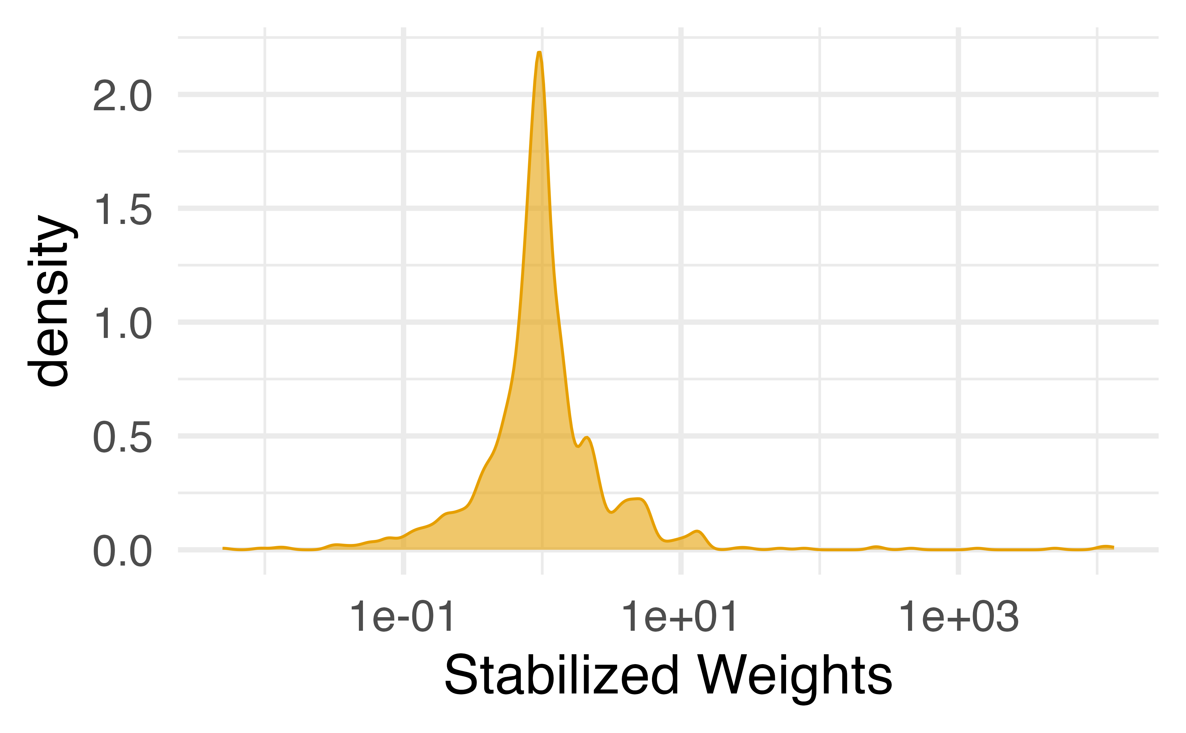
Your Turn 2

Re-fit the above using stabilized weights

03:00

Your Turn 2

wait_times_swts <- post_time_model |>
  augment(data = wait_times) |>
  mutate(swts = wt_ate(
    wait_minutes_posted_avg, 
    .fitted,
    .sigma = .sigma,
    stabilize = TRUE
  ))

Fitting the outcome model

1. Use the stabilized weights in the outcome model. Nothing new here!

lm(
  wt82_71 ~ smkintensity82_71, 
  weights = swts, 
  data = nhefs_swts
) |>
  tidy() |>
  filter(term == "smkintensity82_71") |>
  mutate(estimate = estimate * -10) 

# A tibble: 1 × 5
  term              estimate std.error statistic  p.value
  <chr>                <dbl>     <dbl>     <dbl>    <dbl>
1 smkintensity82_71     1.99    0.0316     -6.30 4.33e-10

Your Turn 3

Estimate the relationship between posted wait times and actual wait times using the stabilized weights we just created.

03:00

Your Turn 3

lm(
  wait_minutes_actual_avg ~ wait_minutes_posted_avg, 
  weights = swts, 
  data = wait_times_swts
) |>
  tidy() |>
  filter(term == "wait_minutes_posted_avg") |>
  mutate(estimate = estimate * 10)

# A tibble: 1 × 5
  term                  estimate std.error statistic p.value
  <chr>                    <dbl>     <dbl>     <dbl>   <dbl>
1 wait_minutes_posted_…     2.39    0.0659      3.63 4.93e-4

Diagnosing issues

1. Extreme weights even after stabilization
2. Bootstrap: non-normal distribution
3. Bootstrap: estimate different from original model

More info

https://github.com/LucyMcGowan/writing-positivity-continous-ps